Amrvis

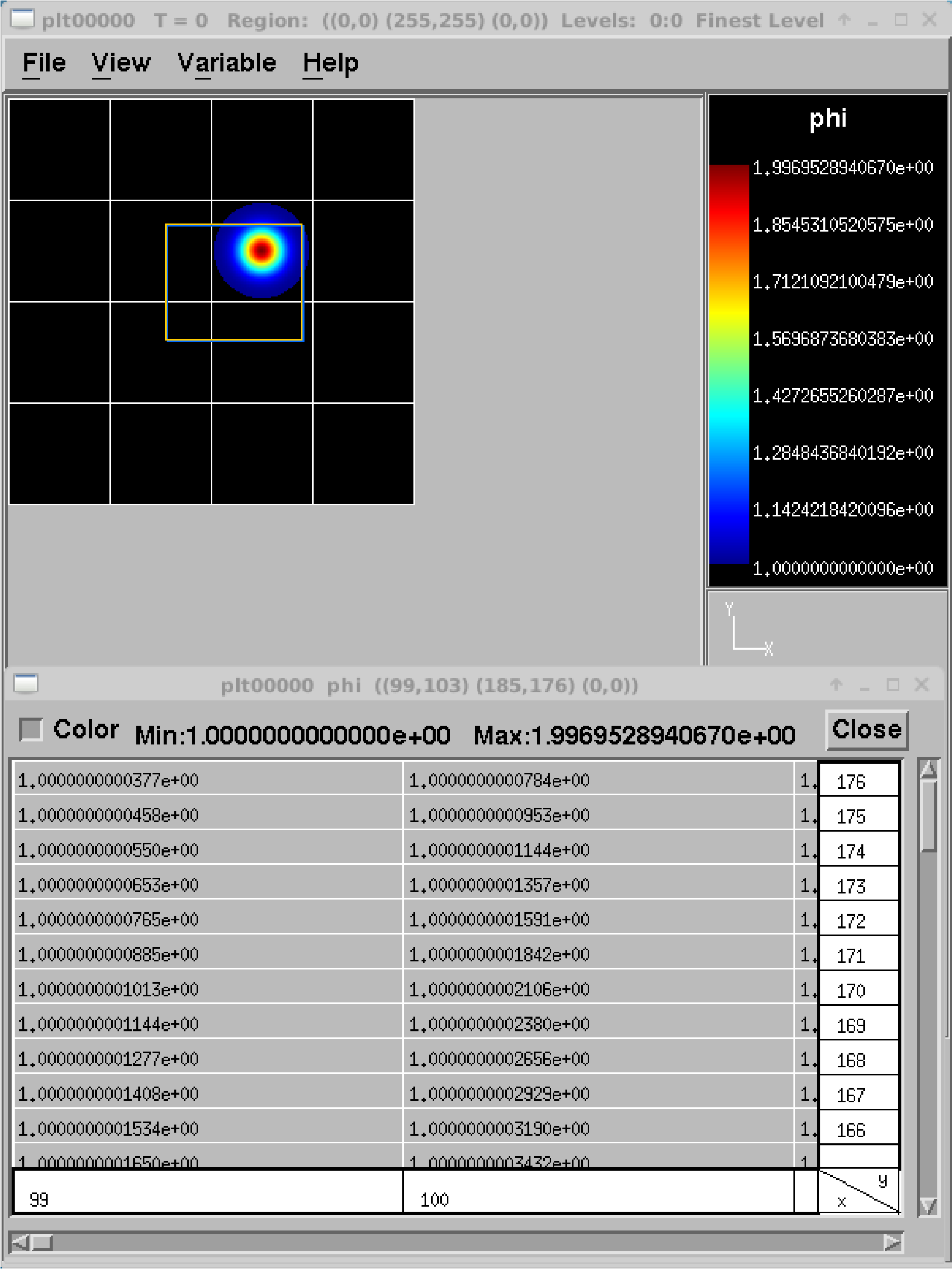
Our favorite visualization tool is Amrvis. We heartily encourage you to build the amrvis1d, amrvis2d, and amrvis3d executables, and use them to visualize your data. A useful feature is View/Dataset, which allows you to view data in a nested spreadsheet that reflects the AMR hierarchy – this can be handy for debugging. Other display options include: the ability to select the number of levels of data to show, whether to display grid boxes, and to specify the color palette. Below are instructions and tips for using Amrvis. Additional information is contained in the document Amrvis/Docs/Amrvis.tex (which can built into a pdf using pdflatex).

Download and Build:

Amrvis is available for download from the AMReX-Codes/Amrvis GitHub repository. To download use,
```
git clone https://github.com/AMReX-Codes/Amrvis
```
To build, cd into Amrvis/, and edit GNUmakefile by setting the variable COMP to your compiler suite.

Type make DIM=1, make DIM=2, or make DIM=3 to build. The result is an executable that looks like amrvis2d.<ver>.ex.

3D Data Visualization with Volpack

If you want to build Amrvis with DIM=3 for display of 3-dimensional data, you must first download and build volpack. This can be done by cloning the repository or via package manager. To install by cloning the repository:
```
git clone https://ccse.lbl.gov/pub/Downloads/volpack.git
```
After downloading, cd into volpack/ and type make.

To install via package manager, it is necessary to install the package, libvolpack1-dev. This package is available for Debian Linux and can be installed with the command:
```
sudo apt install libvolpack1-dev
```
Note

Amrvis requires the OSF/Motif libraries and headers. If you don’t have these you will need to install the development version of motif through your package manager. lesstif gives some functionality and will allow you to build the Amrvis executable, but Amrvis may exhibit subtle anomalies.

On most Linux distributions, the motif library is provided by the openmotif package, and its header files (like Xm.h) are provided by openmotif-devel. If those packages are not installed, then use the OS-specific package management tool to install them.

Note

These instructions assume that the install directories for Amrvis and volpack share the same parent directory. To install volpack in a different location specify the location of volpack in Amrvis’s GNUmakefile by changing the variable VOLPACKDIR to the desired location.

After building you may want to create an alias for convenience. To do this type,
```
alias amrvis2d /tmp/Amrvis/amrvis2d.<ver>.ex
```
Configure:

The settings for Amrvis are saved in the configuration file .amrvis.defaults in your home directory. A default version of this file is available in the parent directory of the Amrvis repo. Run the command cp Amrvis/amrvis.defaults ~/.amrvis.defaults to copy it to your home directory. A color palette is also available in the Amrvis directory as a file named Palette. To configure Amrvis to use this palette you can open the .amrvis.defaults file in your home directory and edit the line containing palette to point to the location of this file. For example,
```
palette     ~/Amrvis/Palette
```
Other lines in .amrvis.defaults control options such as the initial field to display, the number format, window size, etc. If there are multiple instances of the same option, the last option takes precedence.
Run:

By default, the plotfiles are directories that have the form pltXXXXX, where XXXXX is a number corresponding to the timestep that the file was created. Use amrvis2d <filename> or amrvis3d <filename> to see a single plotfile, or for 2D data sets, amrvis2d -a plt*, which will animate the sequence of plotfiles. FArrayBoxes and MultiFabs can also be viewed with the -fab and -mf options. When opening MultiFabs, use the name of the MultiFab’s header file amrvis2d -mf MyMultiFab_H.

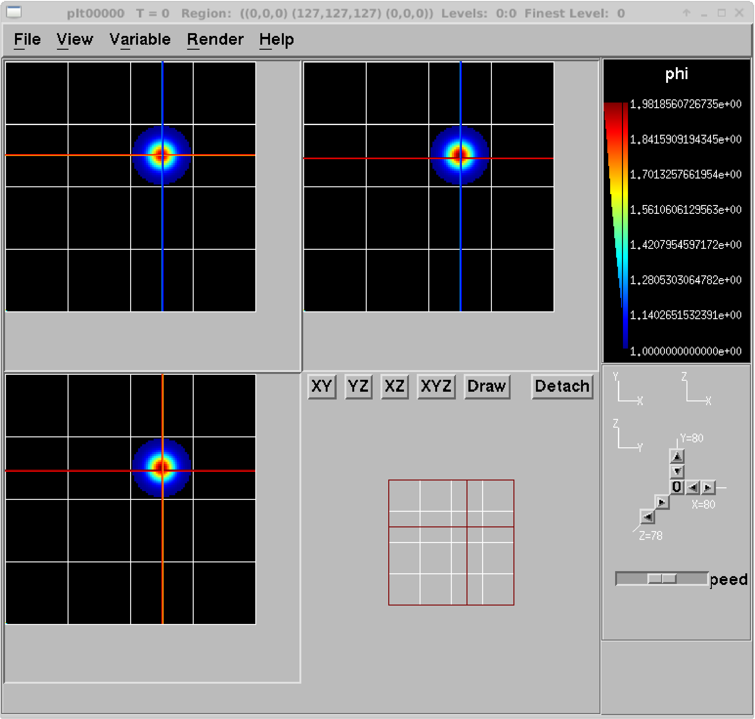
You can use the “Variable” menu to change the variable. You can left-click drag a box around a region and click “View” $\rightarrow$ “Dataset” in order to look at the actual numerical values (see Table 18). Or you can simply left click on a point to obtain the numerical value. You can also export the pictures in several different formats under File/Export. In 2D you can right or center click to get line-out plots. In 3D you can right or center click to change the planes, and hold shift+(right or center) click to get line-out plots.

We have created a number of routines to convert AMReX plotfile data to other formats (such as Matlab), but in order to properly interpret the hierarchical AMR data, each tends to require its own idiosyncrasies. If you would like to display the data in another format, please leave a message on AMReX’s GitHub Discussions page.

Table 18 . 2D and 3D images generated using Amrvis.

Building Amrvis on macOS

As previously outlined at the end of section Building with GNU Make, it is recommended to build using the homebrew package manager to install gcc. Furthermore, you will also need x11 and openmotif. These can be installed using homebrew also:

brew cask install xquartz
brew install openmotif

Note that when the GNUmakefile detects a macOS install, it assumes that dependencies are installed in the locations that Homebrew uses. Namely the /usr/local/ tree for regular dependencies and the /opt/ tree for X11.

VisIt

AMReX data can also be visualized by VisIt, an open source visualization and analysis software. To follow along with this example, first build and run the first heat equation tutorial code (see the section on Example: Heat Equation Solver).

Next, download and install VisIt from https://wci.llnl.gov/simulation/computer-codes/visit. To open a single plotfile, run VisIt, then select “File” $\rightarrow$ “Open file …”, then select the Header file associated with the plotfile of interest (e.g., plt00000/Header). Assuming you ran the simulation in 2D, here are instructions for making a simple plot:

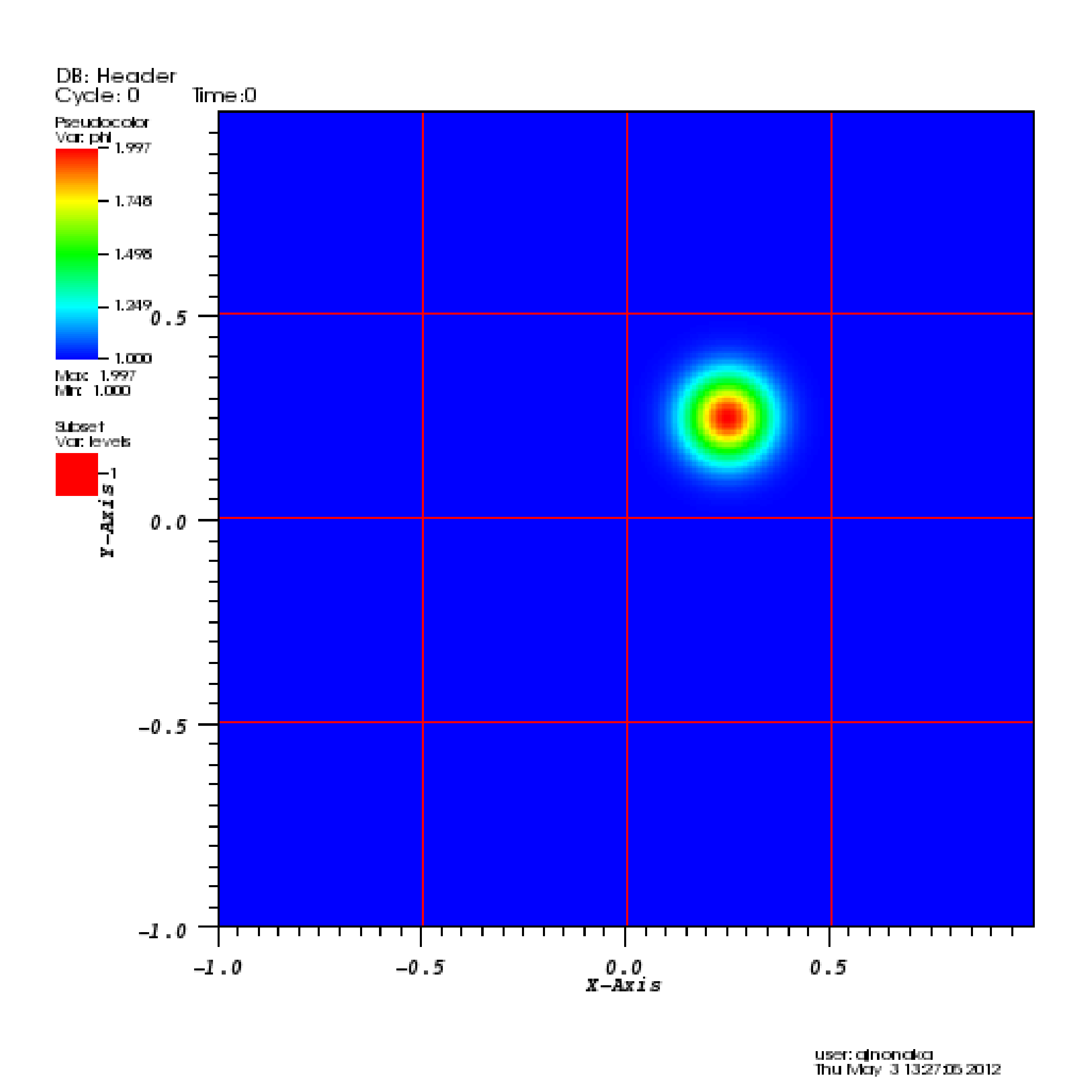
To view the data, select “Add” $\rightarrow$ “Pseudocolor” $\rightarrow$ “phi”, and then select “Draw”.
To view the grid structure (not particularly interesting yet, but when we add AMR it will be), select “Add” $\rightarrow$ “Subset” $\rightarrow$ “levels”. Then double-click the text “Subset - levels”, enable the “Wireframe” option, select “Apply”, select “Dismiss”, and then select “Draw”.
To save the image, select “File” $\rightarrow$ “Set save options”, then customize the image format to your liking, then click “Save”.

Your image should look similar to the left side of Table 19.

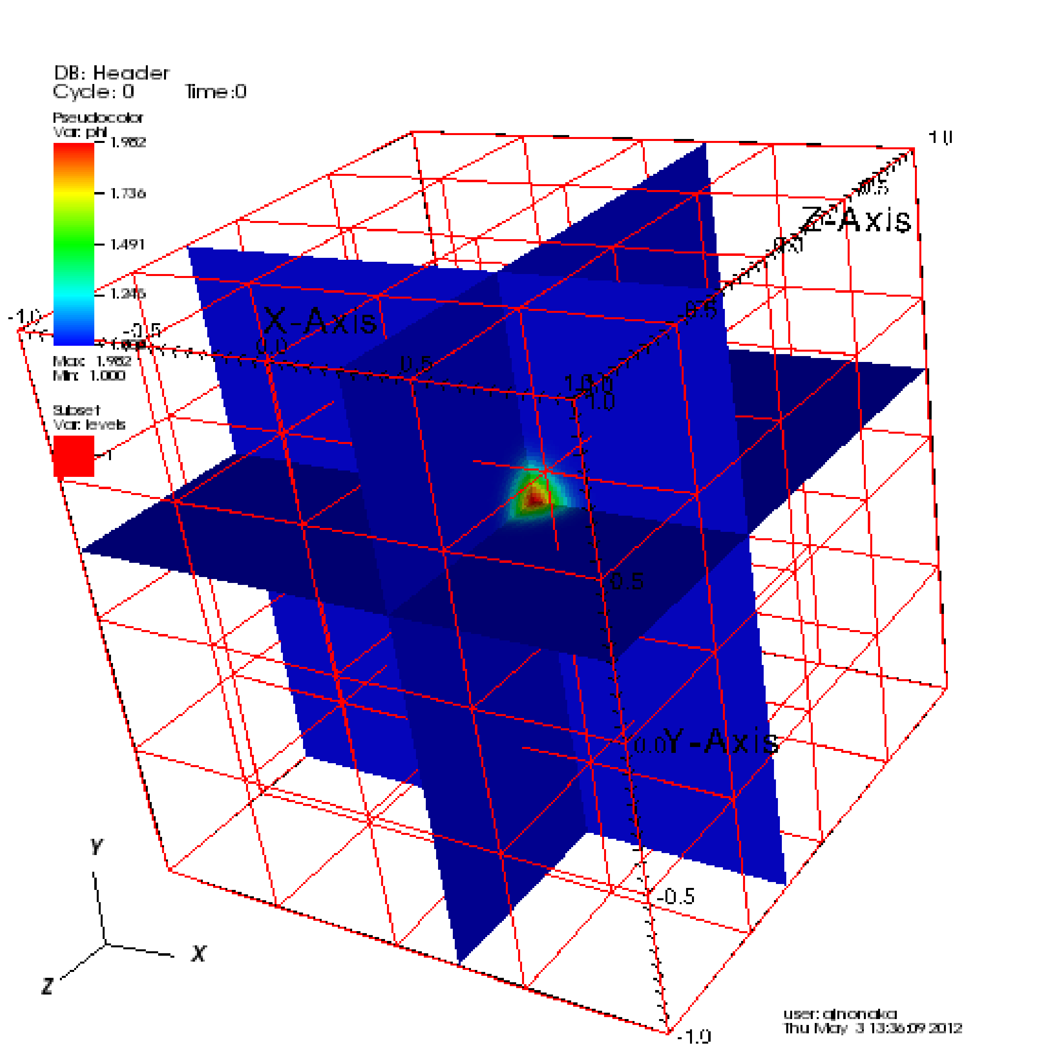
Table 19 : 2D (left) and 3D (right) images generated using VisIt.

In 3D, you must apply the “Operators” $\rightarrow$ “Slicing” $\rightarrow$ “ThreeSlice”, with the “ThreeSlice operator attribute” set to x=0.25, y=0.25, and z=0.25. You can left-click and drag over the image to rotate the image to generate something similar to right side of Table 19.

To make a movie, you must first create a text file named movie.visit with a list of the Header files for the individual frames. This can most easily be done using the command:

~/amrex-tutorials/ExampleCodes/Basic/HeatEquation_EX1_C> ls -1v plt*/Header | tee movie.visit
plt00000/Header
plt01000/Header
plt02000/Header
plt03000/Header
plt04000/Header
plt05000/Header
plt06000/Header
plt07000/Header
plt08000/Header
plt09000/Header
plt10000/Header

The next step is to run VisIt, select “File” $\rightarrow$ “Open file…”, then select movie.visit. Create an image to your liking and press the “play” button on the VCR-like control panel to preview all the frames. To save the movie, choose “File” $\rightarrow$ “Save movie …”, and follow the on-screen instructions.

Warning

The Visit reader determines the value of Cycle from the name of the plotfile (directory), specifically from the integer that follows the string “plt” in the plotfile name. So if you call it plt00100, myplt00100 or this_is_my_plt00100 then it will correctly recognize and print Cycle: 100. If you call it plt00100_old it will also correctly recognize and print Cycle: 100.

However, if you do not have plt followed immediately by the number, e.g. you name it pltx00100, then VisIt will not be able to correctly recognize and print the value for Cycle. (It will still read and display the data itself.)

VisIt HDF5 Format

The plotfiles generated with the HDF5 format can be visualized by VisIt as well. To open a single plotfile, run VisIt, then select “File” $\rightarrow$ “Open file …”, then select the HDF5 plotfile of interest (e.g.,``plt00000.h5``), and select “Chombo” in the “Open file as type” dropdown menu. VisIt can also recognize the time steps automatically based on the numbers in the HDF5 plotfile names in a directory.

ParaView

The open source visualization package ParaView v5.7 and later can be used to view 2D and 3D plotfiles, as well as particles data. Download the package at https://www.paraview.org/.

To open a plotfile (for example, you could run the HeatEquation_EX1_C in 3D):

Run ParaView v5.7, then select “File” $\rightarrow$ “Open”.
Navigate to your run directory, and select the fluid or particle plotfile. Note that you can either open single/multiple plotfile(s) at once by selecting them one by one or select an ensemble of file, labelled as plt.. and indicated as a Group in the “Type” column of the file explorer (see Fig. 16). In the later case, Paraview will load the plotfiles as a time series. ParaView will ask you about the file type – choose “AMReX/BoxLib Grid Reader” or “AMReX/BoxLib Particles Reader”. Note that if your ploftile prefix is not plt or any other type supported by default, then in Files of type you need to first select All files (*).
Under the “Cell Arrays” field, select a variable (e.g., “phi”) and click “Apply”. Note that the default number of refinement levels loaded and visualized is 1. Change to the required number of AMR level before clicking “Apply”.
Under “Representation” select “Surface”.
Under “Coloring” select the variable you chose above.
To add planes, near the top left you will see a cube icon with a green plane slicing through it. If you hover your mouse over it, it will say “Slice”. Click that button.
You can play with the Plane Parameters to define a plane of data to view, as shown in Fig. 14.

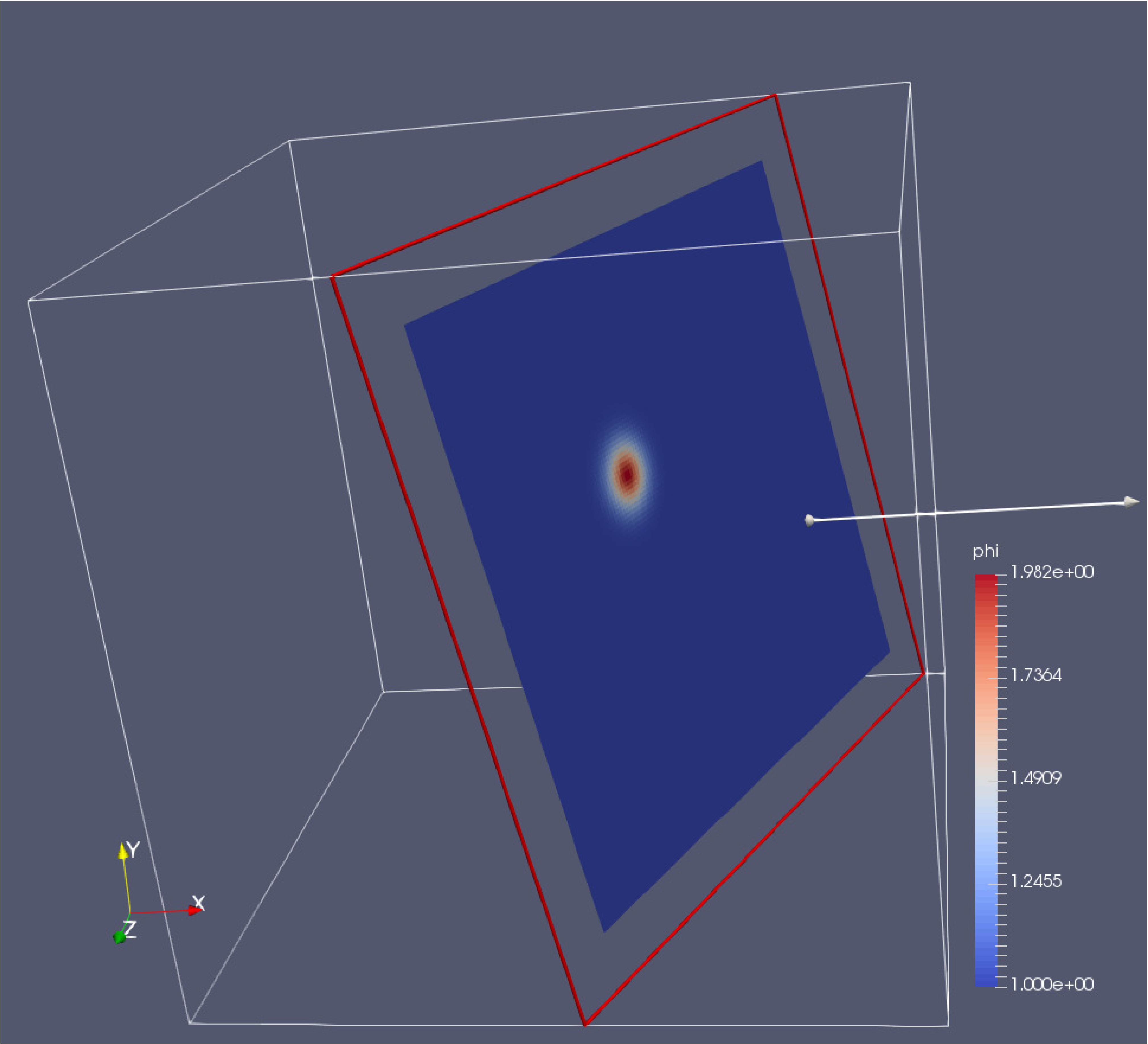
_images/ParaView.png — Fig. 14 : Plotfile image generated with ParaView

Creating and Loading `.series` Files

Another useful feature in ParaView to load and re-load a group of plotfiles is using a .series file (similar to the .visit file in VisIt). It is a text file (say plot_files.series) which lists the plotfiles in a JSON format as below.

{ "file-series-version": "1.0", "files": [
{ "name": "plt00000", "time": 0},
{ "name": "plt00100", "time": 1},
{ "name": "plt00200", "time": 2},
{ "name": "plt00300", "time": 3},
{ "name": "plt00400", "time": 4},
{ "name": "plt00500", "time": 5},
{ "name": "plt00600", "time": 6},
{ "name": "plt00700", "time": 7},
{ "name": "plt00800", "time": 8},
{ "name": "plt00900", "time": 9},
{ "name": "plt01000", "time": 10},] }

write_series_file.sh is a bash script that can generate such a .series file. Navigate to the directory with the plotfiles and save this script. Then run the bash script by executing the following command in the terminal.

bash write_series_file.sh

This will generate a file plot_files.series which indexes the time variable based on the order of the plotfile numbers. Note that if your ploftile prefix is not plt, you can manually edit write_series_file.sh accordingly.

To make a .series file which reads the time out of the plotfile header, use write_series_file_timestamp.sh.

Open ParaView, and then select “File” $\rightarrow$ “Open”. In the “Files of Type” dropdown menu (see Fig. 16) choose the option All Files (*). Then choose plot_files.series and click “OK”. Now the plotfiles have been loaded as a Group as in Step 2 of section ParaView. Now, you can follow the steps 2 to 7 in the section ParaView to plot. As new plotfiles are generated, just re-run the bash script to re-generate the plot_files.series file, right-click on plot_files.series in the ParaView menu, and click on “Reload Files” (see Fig. 15).

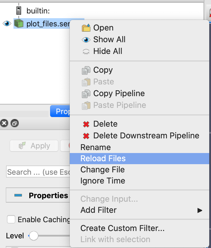
_images/ParaView_series_reload.png — Fig. 15 : File dialog in ParaView showing how to reload a series file

Building an Iso-surface

Note that Paraview is not able to generate iso-surfaces from cell centered data. To build an iso-surface (or iso-line in 2D):

Perform a cell to node interpolation: “Filters” $\rightarrow$ “Alphabetical” $\rightarrow$ “Cell Data to Point Data”.
Use the “Contour” icon (next to the calculator) to select the data from which to build the contour (“Contour by”), enters the iso-surfaces values and click “Apply”.

Visualizing Particle Data

To visualize particle data within plofile directories (for example, you could run the NeighborList example in Tutorials/Particles):

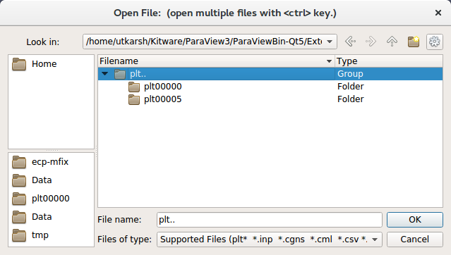
_images/ParaView_filegroup.png — Fig. 16 : File dialog in ParaView showing a group of plotfile directories selected

Run ParaView v5.7, and select then “File” $\rightarrow$ “Open”. You will see a combined “plt..” group. Click on “+” to expand the group, if you want inspect the files in the group. You can select an individual plotfile directory or select a group of directories to read them a time series, as shown in Fig. 16, and click OK. ParaView will ask you about the file type – choose “AMReX/BoxLib Particles Reader”.
The “Properties” panel in ParaView allows you to specify the “Particle Type”, which defaults to “particles”. Using the “Properties” panel, you can also choose which point arrays to read.
Click “Apply” and under “Representation” select “Point Gaussian”.
Change the Gaussian Radius if you like. You can scroll through the frames with the VCR-like controls at the top, as shown in Fig. 17.

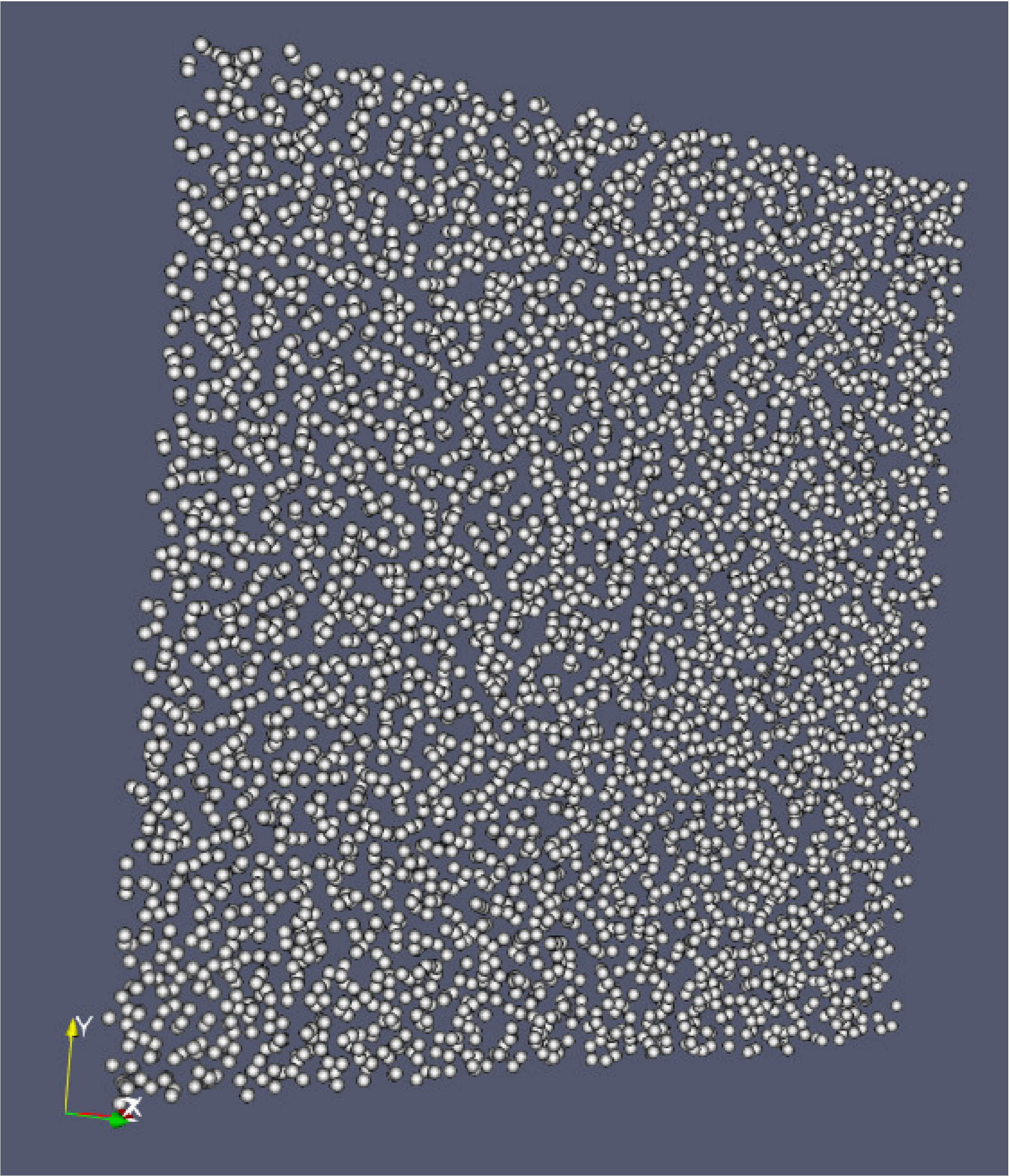
_images/ParaView_particles.png — Fig. 17 : Particle image generated with ParaView

Following these instructions, you can open fluid and/or particles plotfiles and visualize them together on the same Panel View.

Once you have loaded an AMReX plotfile time series (fluid and/or particles), you can generate a movie following these instructions:

“File” $\rightarrow$ “Save Animation…”.
Enter a file name, select “.avi” as the Type of File and click “OK”.
Adjust the resolution, compression and framerate, and click “OK”

Plot a Vector Field

Paraview can be used to plot a vector field from AMR plotfile data. In this example we will assume a single vector has been stored as three separate variables, V_x, V_y and V_z.

The easiest way to create a vector V from the components is to first download the python file makevector.py.

If you are running paraview remotely, put makevector.py in the location of the plotfiles you will open under the heading Remote Plugins.

Now open a plotfile or plotfile group, using File $\rightarrow$ Open. A pop-up will appear, select “AMReX/Boxlib Grid Reader”.
Select the plotfile or group in the Pipeline Browser. The Cell Array Status window of the Properties should populate with the values V_x, V_y and V_z. Select these values and click apply.
Select Tools $\rightarrow$ Manage Plugins... then choose Load New.... Select makevector.py; after you load it you will see makevector in the list of plugins.
Select the MakeVector filter from Filters $\rightarrow$ Alphabetical $\rightarrow$ MakeVector and apply. You will now have the vector V listed with your other variables.

Alternatively, if you prefer not to use the python plugin, you can follow the steps below:

Select the Cell Centers filter from Filters $\rightarrow$ Alphabetical $\rightarrow$ Cell Centers and apply.
Next we’ll define a vector variable using the Calculator filter. Select Filters $\rightarrow$ Alphabetical $\rightarrow$ Calculator. Under the Properties heading, set the Attribute Type to Point Data. The Result Array Name is the name of the vector value we will create. In the line below that we define a new vector value with the equation: V_x*iHat + V_y*jHat + V_z*kHat Note that, the values V_x, V_y and V_z, should be selectable from the dropdown Scalars menu. Apply the filter.

To plot the arrows corresponding to this vector field

Select the Glyph filter, Filters $\rightarrow$ Alphabetical $\rightarrow$ Glyph. Under the heading, Glyph Source, select Arrow. Under Orientation, select the name of the vector value created in the last step. The default name is Result. Apply the filter to display the vector field.

One may want to adjust the appearance of the vector field by scaling each vector by its magnitude. To do this, look under the Scale heading, select the vector value as the Scale Array and select Scale by Magnitude.

To adjust the number and location of vectors displayed, one may alter the settings under the Masking heading.

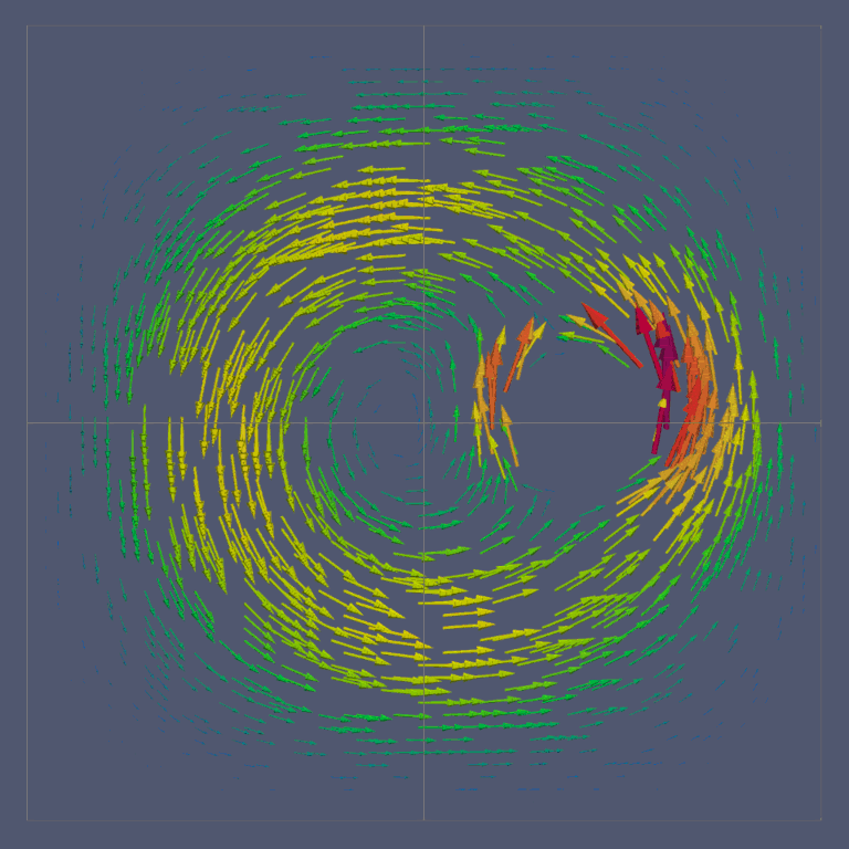
_images/ParaView_vectorfield.png — Fig. 18 Vector Field generated with ParaView

Saving and Loading State Files

Paraview allows users to save the state of their visualization, viz. variable mappings, filters, color maps, etc. The same display style can then be applied to different datasets. See also the Paraview documentation at section 10 and section 8.4.

There are two file formats available for saving and loading state: .pvsm (XML) and .py (Python). Examples of both methods are given below. For these examples, we will be working with the data stored in the folder plt.. that results from running HeatEquation_EX1_C in 3D, as in the example at the beginning of this section.

To save the state of this example, go to File > Save State..., and select the format, location, and name of the state file you want to save. In order to later reload the state you’ve saved, see below.

Note that the Save State option will write state files containing the absolute path to the data files you have loaded. This can cause issues if you’re using state files saved on another machine, have moved your data files, or if Paraview doesn’t know which directory to look in. When loading state from a pvsm file, there are menu options available to navigate to the data source directory. When running a Python script to load data, this can cause an error or crash. We outline the way to avoid this below.

For demonstration purposes, we have also included state files in both formats: slice_state1.pvsm and slice_state1.py

Loading from a Paraview state file (.pvsm)

Go to File > Load State, navigate to slice_state1.pvsm in the file browser and click OK. A new window labeled Load State Options appears with a drop-down menu.
Select Search files under specified directory, and click the ... button to the right of the Data Directory line.
Navigate to amrex-tutorials/ExampleCodes/Basic/HeatEquation_EX1_C/Exec and click OK. This is where the plotfiles will have been saved by default if you’ve built and run the example code HeatEquation_EX1_C.

What you see displayed should be a 2D slice of the solution to the 3D equation.

In general, you can use the load state menu options to navigate to whichever data files you wish to load using your saved pvsm state.

Loading from a Python state file (.py)

In order to load state from a .py file, you must execute the file as a script from the Python Shell within Paraview.

If the Python Shell is not displayed, click the checkbox in View > Python Shell.
Click the Run Script button to the bottom right of the Python shell, navigate to the file amrex/Docs/sphinx_documentation/source/Visualization/slice_state1.py in the file navigator, and click OK.

You should see a 2D slice of the solution to the 3D heat equation. If Paraview reports an error or crashes, see below.

Aside: Working directory in the Paraview Python shell

When you load a state from a Python script in Paraview, it will look in the current working directory of the Python shell to resolve the paths to the data files provided in the Python script.

By default, the current working directory of the Paraview Python shell will be the directory from which you launched Paraview.

Warning

If your Python script makes direct reference to a set of files that can’t be found from your current working directory, then running that script will result in an error, and potentially cause Paraview to crash. This can be addressed by changing the cwd of your Python shell to the proper location.

To check the cwd of the Paraview Python shell, run

>>> import os
>>> os.getcwd()

and make sure that your cwd contains the folder you want to search in so that Python can resolve the path. To change the cwd, run

>>> os.chdir('path/to/folder/containing/your/plotfiles')

Modifying a State File to Work with Different Data

As noted above, a Python state file exported from Paraview will save the path to the data files you used, if any, from your working directory. In order to use such a file with different data, you can modify your Python state file to use the glob package to create a list of potential data file names to search in your current path. The steps are outlined below, including the line numbers in the file slice_state1.py.

Import the glob package
```
4: import glob
```
Create a variable that will hold the list of names to search for. Following the AMReX convention for naming plotfiles, use
```
62: PlotFiles = sorted(glob.glob("plt" + "[0-9]" * 5))
```
In the code section that builds an AMReX/BoxLib Grid Reader, replace the list of data paths with the variable PlotFiles
```
65: plt00000 = AMReXBoxLibGridReader(registrationName="plt00000*", FileNames=PlotFiles)
```
Change the cwd of your Python shell, as outlined above, to a directory containing the other plotfiles you wish to view.
Click Run Script and navigate to the Python state file you wish to run in the pop-up file navigator.

You should now be able to view a new data set with the same filters, color mappings, etc. that you saved to your state file.

ParaView HDF5 Format

The plotfiles generated with the HDF5 format can be visualized by ParaView. To open a single plotfile, run VisIt, select “File” $\rightarrow$ “Open”, then select the HDF5 plotfile (e.g.,``plt00000.h5``). You can select an individual plotfile or select a group of files to read as time series, then click OK. ParaView will ask you about the file type – choose “VisItChomboReader”.

yt

yt, an open source Python package available at http://yt-project.org/, can be used for analyzing and visualizing mesh and particle data generated by AMReX codes. Some of the AMReX developers are also yt project members. Below we describe how to use on both a local workstation, as well as at the NERSC HPC facility for high-throughput visualization of large data sets.

Note - AMReX datasets require yt version 3.4 or greater.

We also note that there is active development of an xarray-like interface for AMReX simulation data via yt; see the xamr docs for more details.

Using on a local workstation

Running yt on a local system generally provides good interactivity, but limited performance. Consequently, this configuration is best when doing exploratory visualization (e.g., experimenting with camera angles, lighting, and color schemes) of small data sets.

To use yt on an AMReX plot file, first start a Jupyter notebook or an IPython kernel, and import the yt module:

In [1]: import yt

In [2]: print(yt.__version__)
3.4-dev

Next, load a plot file; in this example we use a plot file from the Nyx cosmology application:

In [3]: ds = yt.load("plt00401")
yt : [INFO     ] 2017-05-23 10:03:56,182 Parameters: current_time              = 0.00605694344696544
yt : [INFO     ] 2017-05-23 10:03:56,182 Parameters: domain_dimensions         = [128 128 128]
yt : [INFO     ] 2017-05-23 10:03:56,182 Parameters: domain_left_edge          = [ 0.  0.  0.]
yt : [INFO     ] 2017-05-23 10:03:56,183 Parameters: domain_right_edge         = [ 14.24501  14.24501  14.24501]

In [4]: ds.field_list
Out[4]:
[('DM', 'particle_mass'),
 ('DM', 'particle_position_x'),
 ('DM', 'particle_position_y'),
 ('DM', 'particle_position_z'),
 ('DM', 'particle_velocity_x'),
 ('DM', 'particle_velocity_y'),
 ('DM', 'particle_velocity_z'),
 ('all', 'particle_mass'),
 ('all', 'particle_position_x'),
 ('all', 'particle_position_y'),
 ('all', 'particle_position_z'),
 ('all', 'particle_velocity_x'),
 ('all', 'particle_velocity_y'),
 ('all', 'particle_velocity_z'),
 ('boxlib', 'density'),
 ('boxlib', 'particle_mass_density')]

From here one can make slice plots, 3-D volume renderings, etc. An example of the slice plot feature is shown below:

In [9]: slc = yt.SlicePlot(ds, "z", "density")
yt : [INFO     ] 2017-05-23 10:08:25,358 xlim = 0.000000 14.245010
yt : [INFO     ] 2017-05-23 10:08:25,358 ylim = 0.000000 14.245010
yt : [INFO     ] 2017-05-23 10:08:25,359 xlim = 0.000000 14.245010
yt : [INFO     ] 2017-05-23 10:08:25,359 ylim = 0.000000 14.245010

In [10]: slc.show()

In [11]: slc.save()
yt : [INFO     ] 2017-05-23 10:08:34,021 Saving plot plt00401_Slice_z_density.png
Out[11]: ['plt00401_Slice_z_density.png']

The resulting image is Fig. 19. One can also make volume renderings with ; an example is show below:

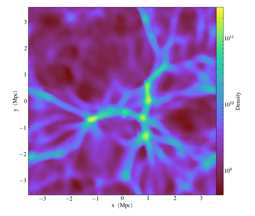
_images/yt_Nyx_density_slice.png — Fig. 19 : Slice plot of $128^3$ Nyx simulation using yt.

In [12]: sc = yt.create_scene(ds, field="density", lens_type="perspective")

In [13]: source = sc[0]

In [14]: source.tfh.set_bounds((1e8, 1e15))

In [15]: source.tfh.set_log(True)

In [16]: source.tfh.grey_opacity = True

In [17]: sc.show()
<Scene Object>:
Sources:
    source_00: <Volume Source>:YTRegion (plt00401): , center=[  1.09888770e+25   1.09888770e+25   1.09888770e+25] cm, left_edge=[ 0.  0.  0.] cm, right_edge=[  2.19777540e+25   2.19777540e+25   2.19777540e+25] cm transfer_function:None
Camera:
    <Camera Object>:
    position:[ 14.24501  14.24501  14.24501] code_length
    focus:[ 7.122505  7.122505  7.122505] code_length
    north_vector:[ 0.81649658 -0.40824829 -0.40824829]
    width:[ 21.367515  21.367515  21.367515] code_length
    light:None
    resolution:(512, 512)
Lens: <Lens Object>:
    lens_type:perspective
    viewpoint:[ 0.95423473  0.95423473  0.95423473] code_length

In [19]: sc.save()
yt : [INFO     ] 2017-05-23 10:15:07,825 Rendering scene (Can take a while).
yt : [INFO     ] 2017-05-23 10:15:07,825 Creating volume
yt : [INFO     ] 2017-05-23 10:15:07,996 Creating transfer function
yt : [INFO     ] 2017-05-23 10:15:07,997 Calculating data bounds. This may take a while.
Set the TransferFunctionHelper.bounds to avoid this.
yt : [INFO     ] 2017-05-23 10:15:16,471 Saving render plt00401_Render_density.png

The output of this is Fig. 20.

_images/yt_Nyx_density_vol_rend.png — Fig. 20 Volume rendering of $128^3$ Nyx simulation using yt. This corresponds to the same plot file used to generate the slice plot in Fig. 19.

Using yt at NERSC (under development)

Because yt is Python-based, it is portable and can be used in many software environments. Here we focus on yt’s capabilities at NERSC, which provides resources for performing both interactive and batch queue-based visualization and analysis of AMReX data. Coupled with yt’s MPI and OpenMP parallelization capabilities, this can enable high-throughput visualization and analysis workflows.

Interactive yt with Jupyter notebooks

Unlike VisIt (see the section on VisIt), yt has no client-server interface. Such an interface is often crucial when one has large data sets generated on a remote system, but wishes to visualize the data on a local workstation. Both copying the data between the two systems, as well as visualizing the data itself on a workstation, can be prohibitively slow.

Fortunately, NERSC has implemented several resources which allow one to interact with yt remotely, emulating a client-server model. In particular, NERSC now hosts Jupyter notebooks which run IPython kernels on the Cori system; this provides users access to the $HOME, /project, and $SCRATCH file systems from a web browser-based Jupyter notebook. *Please note that Jupyter hosting at NERSC is still under development, and the environment may change without notice.*

NERSC also provides Anaconda Python, which allows users to create their own customizable Python environments. It is recommended to install yt in such an environment. One can do so with the following example:

user@cori10:~> module load python/3.5-anaconda
user@cori10:~> conda create -p $HOME/yt-conda numpy
user@cori10:~> source activate $HOME/yt-conda
(/global/homes/u/user/yt-conda/) user@cori10:~> pip install yt

More information about Anaconda Python at NERSC is here: http://www.nersc.gov/users/data-analytics/data-analytics/python/anaconda-python/.

One can then configure this Anaconda environment to run in a Jupyter notebook hosted on the Cori system. Currently this is available in two places: on https://ipython.nersc.gov, and on https://jupyter-dev.nersc.gov. The latter likely reflects what the stable, production environment for Jupyter notebooks will look like at NERSC, but it is still under development and subject to change. To load this custom Python kernel in a Jupyter notebook, follow the instructions at this URL under the “Custom Kernels” heading: http://www.nersc.gov/users/data-analytics/data-analytics/web-applications-for-data-analytics. After writing the appropriate kernel.json file, the custom kernel will appear as an available Jupyter notebook. Then one can interactively visualize AMReX plot files in the web browser. [1]

Parallel

Besides the benefit of no longer needing to move data back and forth between NERSC and one’s local workstation to do visualization and analysis, an additional feature of yt which takes advantage of the computational resources at NERSC is its parallelization capabilities. yt supports both MPI- and OpenMP-based parallelization of various tasks, which are discussed here: http://yt-project.org/doc/analyzing/parallel_computation.html.

Configuring yt for MPI parallelization at NERSC is a more complex task than discussed in the official yt documentation; the command pip install mpi4py is not sufficient. Rather, one must compile mpi4py from source using the Cray compiler wrappers cc, CC, and ftn on Cori. Instructions for compiling mpi4py at NERSC are provided here: http://www.nersc.gov/users/data-analytics/data-analytics/python/anaconda-python/#toc-anchor-3. After mpi4py has been compiled, one can use the regular Python interpreter in the Anaconda environment as normal; when executing yt operations which support MPI parallelization, the multiple MPI processes will spawn automatically.

Although several components of yt support MPI parallelization, a few are particularly useful:

Time series analysis. Often one runs a simulation for many time steps and periodically writes plot files to disk for visualization and post-processing. yt supports parallelization over time series data via the DatasetSeries object. yt can iterate over a DatasetSeries in parallel, with different MPI processes operating on different elements of the series. This page provides more documentation: http://yt-project.org/doc/analyzing/time_series_analysis.html#time-series-analysis.
Volume rendering. yt implements spatial decomposition among MPI processes for volume rendering procedures, which can be computationally expensive. Note that yt also implements OpenMP parallelization in volume rendering, and so one can execute volume rendering with a hybrid MPI+OpenMP approach. See this URL for more detail: http://yt-project.org/doc/visualizing/volume_rendering.html?highlight=openmp#openmp-parallelization.

Generic parallelization over multiple objects. Sometimes one wishes to loop over a series which is not a DatasetSeries, e.g., performing translational or rotational operations on a camera to make a volume rendering in which the field of view moves through the simulation. In this case, one is applying a set of operations on a single object (a single plot file), rather than over a time series of data. For this workflow, yt provides the parallel_objects() function. See this URL for more details: http://yt-project.org/doc/analyzing/parallel_computation.html#parallelizing-over-multiple-objects.

An example of MPI parallelization in yt is shown below, where one animates a time series of plot files from an IAMR simulation while revolving the camera such that it completes two full revolutions over the span of the animation:

import yt
import glob
import numpy as np

yt.enable_parallelism()

base_dir1 = '/global/cscratch1/sd/user/Nyx_run_p1'
base_dir2 = '/global/cscratch1/sd/user/Nyx_run_p2'
base_dir3 = '/global/cscratch1/sd/user/Nyx_run_p3'

glob1 = glob.glob(base_dir1 + '/plt*')
glob2 = glob.glob(base_dir2 + '/plt*')
glob3 = glob.glob(base_dir3 + '/plt*')

files = sorted(glob1 + glob2 + glob3)

ts = yt.DatasetSeries(files, parallel=True)

frame = 0
num_frames = len(ts)
num_revol = 2

slices = np.arange(len(ts))

for i in yt.parallel_objects(slices):
    sc = yt.create_scene(ts[i], lens_type='perspective', field='z_velocity')

    source = sc[0]
    source.tfh.set_bounds((1e-2, 9e+0))
    source.tfh.set_log(False)
    source.tfh.grey_opacity = False

    cam = sc.camera

    cam.rotate(num_revol*(2.0*np.pi)*(i/num_frames),
               rot_center=np.array([0.0, 0.0, 0.0]))

    sc.save(sigma_clip=5.0)

When executed on 4 CPUs on a Haswell node of Cori, the output looks like the following:

user@nid00009:~/yt_vis/> srun -n 4 -c 2 --cpu_bind=cores python make_yt_movie.py
yt : [INFO     ] 2017-05-23 16:51:33,565 Global parallel computation enabled: 0 / 4
yt : [INFO     ] 2017-05-23 16:51:33,565 Global parallel computation enabled: 2 / 4
yt : [INFO     ] 2017-05-23 16:51:33,566 Global parallel computation enabled: 1 / 4
yt : [INFO     ] 2017-05-23 16:51:33,566 Global parallel computation enabled: 3 / 4
P003 yt : [INFO     ] 2017-05-23 16:51:33,957 Parameters: current_time              = 0.103169376949795
P003 yt : [INFO     ] 2017-05-23 16:51:33,957 Parameters: domain_dimensions         = [128 128 128]
P003 yt : [INFO     ] 2017-05-23 16:51:33,957 Parameters: domain_left_edge          = [ 0.  0.  0.]
P003 yt : [INFO     ] 2017-05-23 16:51:33,958 Parameters: domain_right_edge         = [ 6.28318531  6.28318531  6.28318531]
P000 yt : [INFO     ] 2017-05-23 16:51:33,969 Parameters: current_time              = 0.0
P000 yt : [INFO     ] 2017-05-23 16:51:33,969 Parameters: domain_dimensions         = [128 128 128]
P002 yt : [INFO     ] 2017-05-23 16:51:33,969 Parameters: current_time              = 0.0687808060674485
P000 yt : [INFO     ] 2017-05-23 16:51:33,969 Parameters: domain_left_edge          = [ 0.  0.  0.]
P002 yt : [INFO     ] 2017-05-23 16:51:33,969 Parameters: domain_dimensions         = [128 128 128]
P000 yt : [INFO     ] 2017-05-23 16:51:33,970 Parameters: domain_right_edge         = [ 6.28318531  6.28318531  6.28318531]
P002 yt : [INFO     ] 2017-05-23 16:51:33,970 Parameters: domain_left_edge          = [ 0.  0.  0.]
P002 yt : [INFO     ] 2017-05-23 16:51:33,970 Parameters: domain_right_edge         = [ 6.28318531  6.28318531  6.28318531]
P001 yt : [INFO     ] 2017-05-23 16:51:33,973 Parameters: current_time              = 0.0343922351851018
P001 yt : [INFO     ] 2017-05-23 16:51:33,973 Parameters: domain_dimensions         = [128 128 128]
P001 yt : [INFO     ] 2017-05-23 16:51:33,974 Parameters: domain_left_edge          = [ 0.  0.  0.]
P001 yt : [INFO     ] 2017-05-23 16:51:33,974 Parameters: domain_right_edge         = [ 6.28318531  6.28318531  6.28318531]
P000 yt : [INFO     ] 2017-05-23 16:51:34,589 Rendering scene (Can take a while).
P000 yt : [INFO     ] 2017-05-23 16:51:34,590 Creating volume
P003 yt : [INFO     ] 2017-05-23 16:51:34,592 Rendering scene (Can take a while).
P002 yt : [INFO     ] 2017-05-23 16:51:34,592 Rendering scene (Can take a while).
P003 yt : [INFO     ] 2017-05-23 16:51:34,593 Creating volume
P002 yt : [INFO     ] 2017-05-23 16:51:34,593 Creating volume
P001 yt : [INFO     ] 2017-05-23 16:51:34,606 Rendering scene (Can take a while).
P001 yt : [INFO     ] 2017-05-23 16:51:34,607 Creating volume

Because the parallel_objects() function transforms the loop into a data-parallel problem, this procedure strong scales nearly perfectly to an arbitrarily large number of MPI processes, allowing for rapid rendering of large time series of data.

SENSEI

SENSEI is a light weight framework for in situ data analysis. SENSEI’s data model and API provide uniform access to and run time selection of a diverse set of visualization and analysis back ends including VisIt Libsim, ParaView Catalyst, VTK-m, Ascent, ADIOS, Yt, and Python.

System Architecture

_images/sensei_amrex_arch_sm_824.png — Fig. 21 SENSEI’s in situ architecture enables use of a diverse of back ends which can be selected at run time via an XML configuration file

The three major architectural components in SENSEI are data adaptors which present simulation data in SENSEI’s data model, analysis adaptors which present the back end data consumers to the simulation, and bridge code from which the simulation manages adaptors and periodically pushes data through the system. SENSEI comes equipped with a number of analysis adaptors enabling use of popular analysis and visualization libraries such as VisIt Libsim, ParaView Catalyst, Python, and ADIOS to name a few. AMReX contains SENSEI data adaptors and bridge code making it easy to use in AMReX based simulation codes.

SENSEI provides a configurable analysis adaptor which uses an XML file to select and configure one or more back ends at run time. Run time selection of the back end via XML means one user can access Catalyst, another Libsim, yet another Python with no changes to the code. This is depicted in figure Fig. 21. On the left side of the figure AMReX produces data, the bridge code pushes the data through the configurable analysis adaptor to the back end that was selected at run time.

AMReX Integration

AMReX codes based on amrex::Amr can use SENSEI simply by enabling it in the build and run via ParmParse parameters. AMReX codes based on amrex::AmrMesh need to additionally invoke the bridge code in amrex::AmrMeshInSituBridge.

Compiling with GNU Make

For codes making use of AMReX’s build system add the following variable to the code’s main GNUmakefile.

USE_SENSEI_INSITU = TRUE

When set, AMReX’s make files will query environment variables for the lists of compiler and linker flags, include directories, and link libraries. These lists can be quite elaborate when using more sophisticated back ends, and are best set automatically using the sensei_config command line tool that should be installed with SENSEI. Prior to invoking make use the following command to set these variables:

source sensei_config

Typically, the sensei_config tool is in the users PATH after loading the desired SENSEI module. After configuring the build environment with sensei_config, proceed as usual.

make -j4 -f GNUmakefile

Compiling with CMake

For codes making use of AMReX’s CMake based build, one needs to enable SENSEI and point to the CMake configuration installed with SENSEI.

cmake -DAMReX_SENSEI=ON -DSENSEI_DIR=<path to install>/<lib dir>/cmake ..

When CMake generates the make files proceed as usual. Note: <lib dir> may be lib or lib64 or something else depending on what CMake decided to use for your particular OS. See the CMake GNUInstallDirs documentation for more information.

make -j4 -f GNUmakefile

ParmParse Configuration

Once an AMReX code has been compiled with SENSEI features enabled, it will need to be enabled and configured at runtime. This is done using ParmParse input file. The following 3 ParmParse parameters are used:

sensei.enabled = 1
sensei.config = render_iso_catalyst_2d.xml
sensei.frequency = 2

sensei.enabled turns SENSEI on or off. sensei.config points to the SENSEI XML file which selects and configures the desired back end. sensei.frequency controls the number of level 0 time steps in between SENSEI processing.

Back-end Selection and Configuration

The back end is selected and configured at run time using the SENSEI XML file. The XML sets parameters specific to SENSEI and to the chosen back end. Many of the back ends have sophisticated configuration mechanisms which SENSEI makes use of. For example the following XML configuration was used on NERSC’s Cori with IAMR to render 10 iso surfaces, shown in figure Fig. 22, using VisIt Libsim.

<sensei>
  <analysis type="libsim" frequency="1" mode="batch"
    visitdir="/usr/common/software/sensei/visit"
    session="rt_sensei_configs/visit_rt_contour_alpha_10.session"
    image-filename="rt_contour_%ts" image-width="1555" image-height="815"
    image-format="png" enabled="1"/>
</sensei>

The session attribute names a session file that contains VisIt specific runtime configuration. The session file is generated using VisIt GUI on a representative dataset. Usually this data set is generated in a low resolution run of the desired simulation.

_images/rt_2048_visit_000500.png — Fig. 22 SENSEI-Libsim in situ visualization of a Raleigh-Taylor instability computed by IAMR on NERSC Cori using 2048 cores.

The same run and visualization was repeated using ParaView Catalyst, shown in figure Fig. 23, by providing the following XML configuration.

<sensei>
  <analysis type="catalyst" pipeline="pythonscript"
    filename="rt_sensei_configs/rt_contour.py" enabled="1" />
</sensei>

Here the filename attribute is used to pass Catalyst a Catalyst specific configuration that was generated using the ParaView GUI on a representative dataset.

_images/rt_2048_paraview_000500.png — Fig. 23 SENSEI-Catalyst in situ visualization of a Raleigh-Taylor instability computed by IAMR on NERSC Cori using 2048 cores.

Obtaining SENSEI

SENSEI is hosted on github at https://github.com/SENSEI-insitu/SENSEI.git

To ease the burden of wrangling back end installs SENSEI provides two platforms with all dependencies pre-installed, a VirtualBox VM, and a NERSC Cori deployment. New users are encouraged to experiment with one of these.

SENSEI VM

The SENSEI VM comes with all of SENSEI’s dependencies and the major back ends such as VisIt and ParaView installed. The VM is the easiest way to test things out. It also can be used to see how installs were done and the environment configured.

NERSC Cori

SENSEI is deployed at NERSC on Cori. The NERSC deployment includes the major back ends such as ParaView Catalyst, VisIt Libsim, and Python.

AmrLevel Tutorial with Catalyst

The following steps show how to run the tutorial with ParaView Catalyst. The simulation will periodically write images during the run.

ssh cori.nersc.gov
cd $SCRATCH
git clone https://github.com/AMReX-Codes/amrex.git
git clone https://github.com/AMReX-Codes/amrex-tutorials.git
cd amrex-tutorials/ExampleCodes/Amr/Advection_AmrLevel/Exec/SingleVortex
module use /usr/common/software/sensei/modulefiles
module load sensei/2.1.0-catalyst-shared
source sensei_config
vim GNUmakefile
# USE_SENSEI_INSITU=TRUE
make -j4 -f GNUmakefile
vim inputs
# sensei.enabled=1
# sensei.config=sensei/render_iso_catalyst_2d.xml
salloc -C haswell -N 1 -t 00:30:00 -q debug
cd $SCRATCH/amrex-tutorials/ExampleCodes/Amr/Advection_AmrLevel/Exec/SingleVortex
./main2d.gnu.haswell.MPI.ex inputs

AmrLevel Tutorial with Libsim

The following steps show how to run the tutorial with VisIt Libsim. The simulation will periodically write images during the run.

ssh cori.nersc.gov
cd $SCRATCH
git clone https://github.com/AMReX-Codes/amrex.git
git clone https://github.com/AMReX-Codes/amrex-tutorials.git
cd amrex-tutorials/ExampleCodes/Amr/Advection_AmrLevel/Exec/SingleVortex
module use /usr/common/software/sensei/modulefiles
module load sensei/2.1.0-libsim-shared
source sensei_config
vim GNUmakefile
# USE_SENSEI_INSITU=TRUE
make -j4 -f GNUmakefile
vim inputs
# sensei.enabled=1
# sensei.config=sensei/render_iso_libsim_2d.xml
salloc -C haswell -N 1 -t 00:30:00 -q debug
cd $SCRATCH/amrex-tutorials/ExampleCodes/Amr/Advection_AmrLevel/Exec/SingleVortex
./main2d.gnu.haswell.MPI.ex inputs