Embedded Boundaries
For computations with complex geometries, AMReX provides data structures and algorithms to employ an embedded boundary (EB) approach to PDE discretizations. In this approach, the underlying computational mesh is uniform and block-structured, but the boundary of the irregular-shaped computational domain conceptually cuts through this mesh. Each cell in the mesh becomes labeled as regular, cut or covered, and the finite-volume based discretization methods traditionally used in AMReX applications can be modified to incorporate these cell shapes. See Fig. 11 for an illustration.
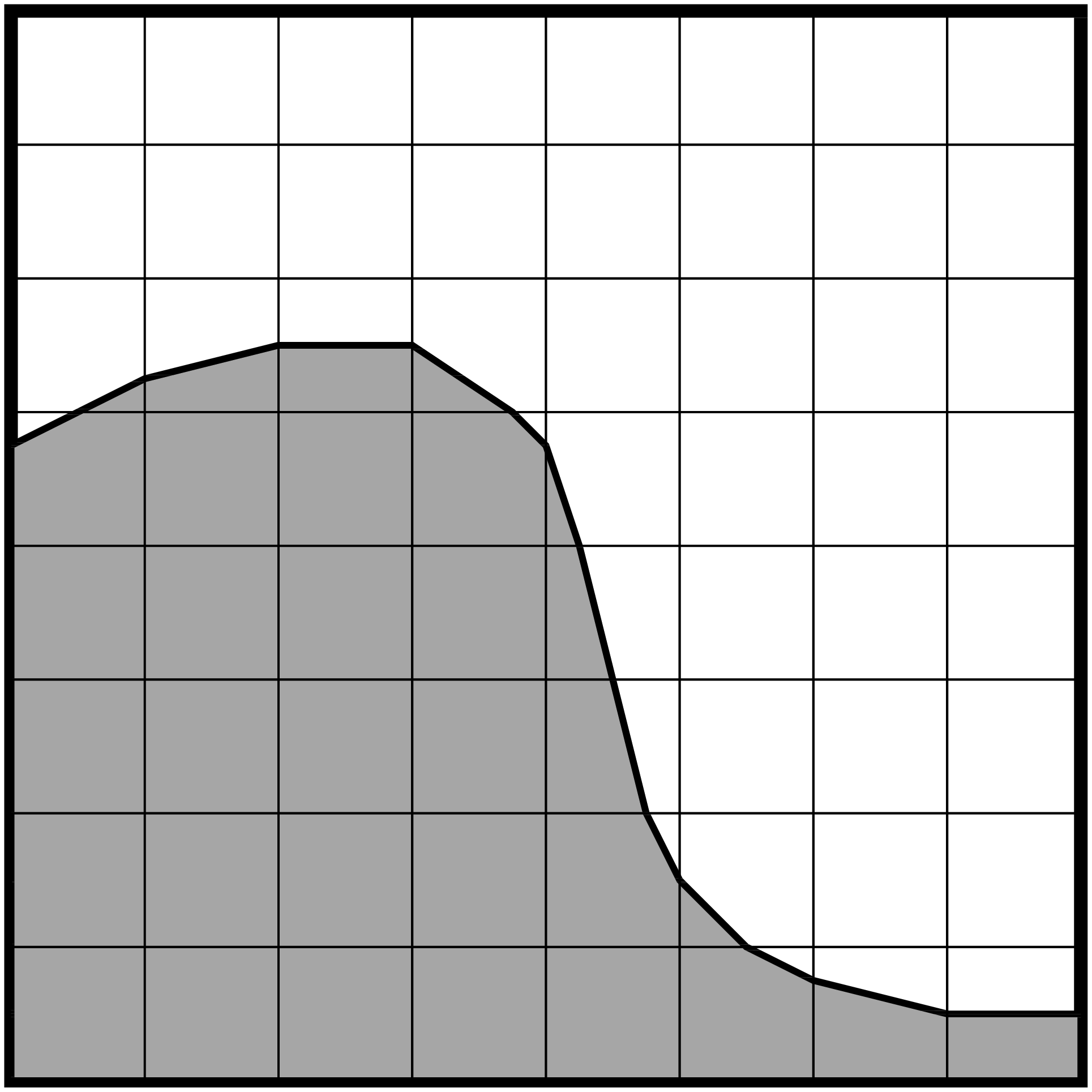
Fig. 11 In the embedded boundary approach to discretizing PDEs, the (uniform) rectangular mesh is cut by the irregular shape of the computational domain. The cells in the mesh are labeled as regular, cut, or covered.
Note that in a completely general implementation of the EB approach, there would be no restrictions on the shape or complexity of the EB surface. With this generality comes the possibility that the process of “cutting” the cells results in a single \((i,j,k)\) cell being broken into multiple cell fragments. The current release of AMReX does not support multi-valued cells, thus there is a practical restriction on the complexity of domains (and numerical algorithms) supported.
AMReX’s relatively simple grid generation technique allows computational meshes for rather complex geometries to be generated quickly and robustly. However, the technique can produce arbitrarily small cut cells in the domain. In practice, such small cells can have significant impact on the robustness and stability of traditional finite volume methods. The redistribution section in AMReX-Hydro’s documentation provides an overview of the finite volume discretization in an embedded boundary cell and a class of approaches to deal with this “small cell” problem in a robust and efficient way.
This chapter discusses the EB tools, data structures and algorithms currently supported by AMReX to enable the construction of discretizations of conservation law systems. The discussion will focus on general requirements associated with building fluxes and taking divergences of them to advance such systems. We also give examples of how to initialize the geometry data structures and access them to build the numerical difference operators. Finally, we present EB support for linear solvers.