The Particle

The particle classes can be used by including the header AMReX_Particles.H. The most basic particle data structure is the particle itself:

Particle<3, 2> p;

This is a templated data type, designed to allow flexibility in the number and type of components that the particles carry. The first template parameter is the number of extra Real variables this particle will have (either single or double precision [1]), while the second is the number of extra integer variables. It is important to note that this is the number of extra real and integer variables; a particle will always have at least AMREX_SPACEDIM real components that store the particle’s position and one 64-bit integer component that stores a combination of the particle’s unique id and cpu numbers.

The particle struct is stored such that the Real components come first and the integer component second. Additionally, the required particle variables are stored before the optional ones, for both the real and the integer components. For example, say we want to define a particle type that stores a mass, three velocity components, and two extra integer flags. Our particle struct would be declared like:

Particle<4, 2> p;

and the order of the particle components in would be (assuming AMREX_SPACEDIM is 3): x y z m vx vy vz idcpu flag1 flag2. [2]

The idcpu variable stores a combination of the MPI process a particle was generated on (the cpu) and an identification number that is specific to that process (the id). The combination of these numbers is unique across processes. This is done to facilitate the creation of particle initial conditions in parallel. In storing these identifying numbers, 39 bits are devoted to the id, allowing approximately 550 billion possible local id numbers, and 24 bits are used to store the cpu, allowing about 16.8 million unique (MPI) processes.

One bit is devoted to mark a particle valid or invalid. This is often used to remove particles from a simulation. During Redistribute(), particles with invalid ids are removed from the simulation by default, although this behavior is customizable. Particles with invalid ids are also not written out during plotfile writes or checkpoint / restart operations. The allowed values for p.id() are 0 to 2**39 - 1, and the allowed values for p.cpu() are 0 to 2**24 - 1.

To pack and unpack these numbers, one uses the following syntax:

Particle <0, 0> p;
p.id() = 1;
p.cpu() = 0;
amrex::Print() << p.m_idcpu << "\n"; // 9223372036871553024
amrex::Print() << p.id() << " " << p.cpu() << "\n"; // 1 0

Setting Particle data

The Particle struct provides a number of methods for getting and setting a particle’s data. For the required particle components, there are special, named methods. For the “extra” real and integer data, you can use the rdata and idata methods, respectively.

Particle<2, 2> p;

p.pos(0) = 1.0;
p.pos(1) = 2.0;
p.pos(2) = 3.0;
p.id() = 1;
p.cpu()  = 0;

// p.rdata(0) is the first extra real component, not the
// first real component overall
p.rdata(0) = 5.0;
p.rdata(1) = 5.0;

// and likewise for p.idata(0);
p.idata(0) = 17;
p.idata(1) = -64;

The ParticleContainer

One particle by itself is not very useful. To do real calculations, a collection of particles needs to be defined, and the location of the particles within the AMR hierarchy (and the corresponding MPI process) needs to be tracked as the particle positions change. To do this, we provide the ParticleContainer class:

using MyParticleContainer = ParticleContainer<3, 2, 4, 4>;
MyParticleContainer mypc;

Like the Particle class itself, the ParticleContainer class is templated. The first two template parameters have the same meaning as before: they define the number of each type of variables that the particles in this container will store. Particles added to the container are stored in the Array-of-Structs style. In addition, there are two more optional template parameters that allow the user to specify additional particle variables that will be stored in Struct-of-Arrays form.

Arrays-of-Structs and Structs-of-Arrays

The difference between Array-of-Structs (AoS) and Struct-of-Arrays (SoA) data is in how the data is laid out in memory. For the AoS data, all the variables associated with particle 1 are next to each other in memory, followed by all the variables associated with particle 2, and so on. For variables stored in SoA style, all the particle data for a given component is next to each other in memory, and each component is stored in a separate array. For convenience, we (arbitrarily) refer to the components in the particle struct as particle data, and components stored in the Struct-of-Arrays as particle attributes. See the figure below for an illustration.

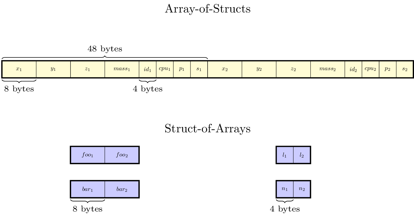
Fig. 8 An illustration of how the particle data for a single tile is arranged in memory. This particle container has been defined with NStructReal = 1, NStructInt = 2, NArrayReal = 2, and NArrayInt = 2. In this case, each tile in the particle container has five arrays: one with the particle struct data, two additional real arrays, and two additional integer arrays. In the tile shown, there are only 2 particles. We have labelled the extra real data member of the particle struct to be mass, while the extra integer members of the particle struct are labeled p, and s, for “phase” and “state”. The variables in the real and integer arrays are labelled foo, bar, l, and n, respectively. We have assumed that the particles are double precision.

Attention

The ability to store particle data in AoS form is provided for backward compatibility and convenience; however, for performance reasons, whether targeting CPU or GPU execution, we recommend storing extra particle variables in SoA form. Additionally, starting in AMReX version 23.05, the ability to store all particle data, including the particle positions and idcpu numbers, is provided via the amrex::ParticleContainerPureSoA class. Details on using pure SoA particles are provided in the Section on Pure Struct-of-Array Particles.

Constructing ParticleContainers

A particle container is always associated with a particular set of AMR grids and a particular set of DistributionMaps that describes which MPI processes those grids live on. For example, if you only have one level, you can define a ParticleContainer to store particles on that level using the following constructor:

ParticleContainer (const Geometry            & geom,
                   const DistributionMapping & dmap,
                   const BoxArray            & ba);

Or, if you have multiple levels, you can use following constructor instead:

ParticleContainer (const Vector<Geometry>            & geom,
                   const Vector<DistributionMapping> & dmap,
                   const Vector<BoxArray>            & ba,
                   const Vector<int>                 & rr);

Note the set of grids used to define the ParticleContainer doesn’t have to be the same set used to define the simulation’s mesh data. However, it is often desirable to have the two hierarchies track each other. If you are using an AmrCore class in your simulation (see the Chapter on AmrCore Source Code), you can achieve this by using the AmrParticleContainer class. The constructor for this class takes a pointer to your AmrCore derived class, instead:

AmrTracerParticleContainer (AmrCore* amr_core);

In this case, the Vector<BoxArray> and Vector<DistributionMap> used by your ParticleContainer will be updated automatically to match those in your AmrCore.

The ParticleTile

The ParticleContainer stores the particle data in a manner prescribed by the set of AMR grids used to define it. Local particle data is always stored in a data structure called a ParticleTile, which contains a mixture of AoS and SoA components as described above. The tiling behavior of ParticleTile is determined by the parameter, particle.do_tiling:

• If particles.do_tiling=0, then there is always exactly one ParticleTile per grid. This is equivalent to setting a very large particles.tile_size in each direction.

• If particles.do_tiling=1, then each grid can have multiple ParticleTile objects associated with it based on the particles.tile_size parameter.

The AMR grid to which a particle is assigned, is determined by examining its position and binning it, using the domain left edge as an offset. By default, a particle is assigned to the finest level that contains its position, although this behavior can be tweaked if desired.

Note

ParticleTile data tiling with MFIter behaves differently than mesh data. With mesh data, the tiling is strictly logical –the data is laid out in memory the same way whether tiling is turned on or off. With particle data, however, the particles are actually stored in different arrays when tiling is enabled. As with mesh data, the particle tile size can be tuned so that an entire tile’s worth of particles will fit into a cache line at once.

Redistribute

Once the particles move, their data may no longer be in the right place in the container. They can be reassigned by calling the Redistribute() method of ParticleContainer. After calling this method, all the particles will be moved to their proper places in the container, and all invalid particles (particles with id set to -1) will be removed. All the MPI communication needed to do this happens automatically.

Application codes will likely want to create their own derived ParticleContainer class that specializes the template parameters and adds additional functionality, like setting the initial conditions, moving the particles, etc. See the particle tutorials for examples of this. .. particle tutorials: https://amrex-codes.github.io/amrex/tutorials_html/Particles_Tutorial.html

Initializing Particle Data

In the following code snippet, we demonstrate how to set particle initial conditions for both SoA and AoS data. We loop over all the tiles using MFIter, and add as many particles as we want to each one.

for (MFIter mfi = MakeMFIter(lev); mfi.isValid(); ++mfi) {

    // ``particles'' starts off empty
    auto& particles = GetParticles(lev)[std::make_pair(mfi.index(),
                                        mfi.LocalTileIndex())];

    ParticleType p;
    p.id()   = ParticleType::NextID();
    p.cpu()  = ParallelDescriptor::MyProc();
    p.pos(0) = ...
    etc...

    // AoS real data
    p.rdata(0) = ...
    p.rdata(1)  = ...

    // AoS int data
    p.idata(0) = ...
    p.idata(1) = ...

    // Particle real attributes (SoA)
    std::array<double, 2> real_attribs;
    real_attribs[0] = ...
    real_attribs[1] = ...

    // Particle int attributes (SoA)
    std::array<int, 2> int_attribs;
    int_attribs[0] = ...
    int_attribs[1]  = ...

    particles.push_back(p);
    particles.push_back_real(real_attribs);
    particles.push_back_int(int_attribs);

    // ... add more particles if desired ...
  }

Often, it makes sense to have each process only generate particles that it owns, so that the particles are already in the right place in the container. In general, however, users may need to call Redistribute() after adding particles, if the processes generate particles they don’t own (for example, if the particle positions are perturbed from the cell centers and thus end up outside their parent grid).

Note

The above code snippet, which successively calls push_back on the particle vectors, assumes you have compiled AMReX for CPU execution. For GPU codes, one can either generate particles on the host and copy them to the device, or generate the particles directly on the GPU. For the first approach, please see the sample code here. For an example of generating a variable number of particles in each cell directly on the GPU, please see this Electromagnetic Particle-in-Cell tutorial

Adding particle components at runtime

In addition to the components specified as template parameters, you can also add additional Real and int components at runtime. These components will be stored in Struct-of-Array style. To add a runtime component, use the AddRealComp and AddIntComp methods of ParticleContainer, like so:

const bool communicate_this_comp = true;
for (int i = 0; i < num_runtime_real; ++i)
{
    AddRealComp(communicate_this_comp);
}
for (int i = 0; i < num_runtime_int; ++i)
{
    AddIntComp(communicate_this_comp);
}

Runtime-added components can be accessed like regular Struct-of-Array data. The new components will be added at the end of the compile-time defined ones.

When you are using runtime components, it is crucial that when you are adding particles to the container, you call the DefineAndReturnParticleTile method for each tile prior to adding any particles. This will make sure the space for the new components has been allocated. For example, in the above section on initializing particle data, we accessed the particle tile data using the GetParticles method. If we runtime components are used, DefineAndReturnParticleTile should be used instead:

for(MFIter mfi = MakeMFIter(lev); mfi.isValid(); ++mfi)
{
    // instead of this...
    // auto& particles = GetParticles(lev)[std::make_pair(mfi.index(),
    //                                     mfi.LocalTileIndex())];

    // we do this...
    auto& particle_tile = DefineAndReturnParticleTile(lev, mfi);

    // add particles to particle_tile as above...
}

Iterating over Particles

To iterate over the particles on a given level in your container, you can use the ParIter class, which comes in both const and non-const flavors. For example, to iterate over all the AoS data:

using MyParConstIter = MyParticleContainer::ParConstIterType;
for (MyParConstIter pti(pc, lev); pti.isValid(); ++pti) {
    const auto& particles = pti.GetArrayOfStructs();
    for (const auto& p : particles) {
        // do stuff with p...
    }
}

The outer loop will execute once every grid (or tile, if tiling is enabled) that contains particles; grids or tiles that don’t have any particles will be skipped. You can also access the SoA data using the \(ParIter\) as follows:

using MyParIter = MyParticleContainer::ParIterType;
for (MyParIter pti(pc, lev); pti.isValid(); ++pti) {
    auto& particle_attributes = pti.GetStructOfArrays();
    RealVector& real_comp0 = particle_attributes.GetRealData(0);
    IntVector&  int_comp1  = particle_attributes.GetIntData(1);
    for (int i = 0; i < pti.numParticles; ++i) {
        // do stuff with your SoA data...
    }
}

Passing particle data into Fortran routines

Because the AMReX particle struct is a Plain-Old-Data type, it is interoperable with Fortran when the bind(C) attribute is used. It is therefore possible to pass a grid or tile worth of particles into fortran routines for processing, instead of iterating over them in C++. You can also define a Fortran derived type that is equivalent to C struct used for the particles. For example:

use amrex_fort_module, only: amrex_particle_real
use iso_c_binding ,    only: c_int

type, bind(C)  :: particle_t
   real(amrex_particle_real) :: pos(3)
   real(amrex_particle_real) :: vel(3)
   real(amrex_particle_real) :: acc(3)
   integer(c_int64_t) :: idcpu
end type particle_t

is equivalent to a particle struct you get with Particle<6, 0>. Here, amrex_particle_real is either single or doubled precision, depending on whether USE_SINGLE_PRECISION_PARTICLES is TRUE or not. We recommend always using this type in Fortran routines that work on particle data to avoid hard-to-debug incompatibilities between floating point types.

Pure Struct-of-Array Particles

Beginning with AMReX version 24.05, the requirement that the particle positions and ids be stored in AoS form has been lifted. Users can now use the class amrex::ParticleContainerPureSoA, which stores all components in SoA form. When using data layout, it is assumed that the first AMREX_SPACEDIM Real components store the particle position variables, which are used internally to map particle coordinates to grids and cells.

For the most part, functions that work on the standard ParticleContainer will also work on ParticleContainerPureSoA. ParticleTile can be used to access the underlying StructOfArrays, which can be used as before. However, it is particlularly convenient to use the [] operator of ParticleTileData, which allows the same code to work with both AoS and pure SoA particles. For example, within a ParIter loop, one can do:

// Iterating over SoA Particles
ParticleTileDataType ptd = pti.GetParticleTile().getParticleTileData();

ParallelFor( np, [=] AMREX_GPU_DEVICE (long ip)
{
    ParticleType p = ptd[ip];  // p will be a different type for AoS and pure SoA
    // use p.pos(0), p.id(), etc.
}

In this way, code can be written that is agnostic as to the data layout. For more examples of pure SoA particles, please see the SOA tests in amrex/Tests/Particles/, or refer to WarpX, Hipace++, or ImpactX, which use this type of particle container.

Interacting with Mesh Data

It is common to want to have the mesh communicate information to the particles and vice versa. For example, in Particle-in-Cell calculations, the particles deposit their charges onto the mesh, and later, the electric fields computed on the mesh are interpolated back to the particles.

To help perform these sorts of operations, we provide the ParticleToMesh and MeshToParticles functions. These functions operate on an entire ParticleContainer at once, interpolating data back and forth between an input MultiFab. A user-provided lambda function is passed in that specifies the kind of interpolation to perform. Any needed parallel communication (from particles that contribute some of their weight to guard cells, for example) is performed internally. Additionally, these methods support both a single-grid (the particles and the mesh use the same boxes and distribution mappings) and dual-grid (the particles and mesh have different layouts) formalism. In the latter case, the needed parallel communication is also performed internally.

We show examples of these types of operations below. The first snippet shows how to deposit a particle quantiy from the first real component of the particle data to the first component of a MultiFab using linear interpolation.

const auto plo = geom.ProbLoArray();
const auto dxi = geom.InvCellSizeArray();
amrex::ParticleToMesh(myPC, partMF, 0,
                      [=] AMREX_GPU_DEVICE (const MyParticleContainer::ParticleTileType::ConstParticleTileDataType& ptd, int i,
                                            amrex::Array4<amrex::Real> const& rho)
    {
        auto p = ptd[i];
        ParticleInterpolator::Linear interp(p, plo, dxi);

        interp.ParticleToMesh(p, rho, 0, 0, 1,
                    [=] AMREX_GPU_DEVICE (const MyParticleContainer::ParticleType& part, int comp)
                    {
                        return part.rdata(comp);
                    });
    });

The inverse operation, in which the particles communicate data to the mesh, is quite similar:

amrex::MeshToParticle(myPC, acceleration, 0,
    [=] AMREX_GPU_DEVICE (MyParticleContainer::ParticleType& p,
                          amrex::Array4<const amrex::Real> const& acc)
    {
        ParticleInterpolator::Linear interp(p, plo, dxi);

        interp.MeshToParticle(p, acc, 0, 1+AMREX_SPACEDIM, AMREX_SPACEDIM,
                [=] AMREX_GPU_DEVICE (amrex::Array4<const amrex::Real> const& arr,
                                      int i, int j, int k, int comp)
                {
                    return arr(i, j, k, comp);  // no weighting
                },
                [=] AMREX_GPU_DEVICE (MyParticleContainer::ParticleType& part,
                                      int comp, amrex::Real val)
                {
                    part.rdata(comp) += ParticleReal(val);
                });
    });

In this case, we linearly interpolate AMREX_SPACEDIM values starting from the 0th component of the input MultiFab to the particles, writing them starting at particle component 1. Note that ParticleInterpolator::MeshToParticle takes two lambda functions, one that generates the particle quantity to interpolate and another that shows how to update the mesh value.

Finally, the snippet below shows how to use this function to simply count the number of particles in each cell (i.e. to deposit using “nearest neighbor” interpolation)

amrex::ParticleToMesh(myPC, partiMF, 0,
 [=] AMREX_GPU_DEVICE (const MyParticleContainer::SuperParticleType& p,
                       amrex::Array4<int> const& count)
 {
     ParticleInterpolator::Nearest interp(p, plo, dxi);

     interp.ParticleToMesh(p, count, 0, 0, 1,
         [=] AMREX_GPU_DEVICE (const MyParticleContainer::ParticleType& /*p*/, int /*comp*/) -> int
         {
             return 1;  // just count the particles per cell
         });
 });

For more complex examples of interacting with mesh data, we refer readers to our Electromagnetic PIC tutorial

Or, for a complete example of an electrostatic PIC calculation that includes static mesh refinement, please see the Electrostatic PIC tutorial.

Short Range Forces

In a PIC calculation, the particles don’t interact with each other directly; they only see each other through the mesh. An alternative use case is particles that exert short-range forces on each other. In this case, beyond some cut-off distance, the particles don’t interact with each other and therefore don’t need to be included in the force calculation. Our approach to these kind of particles is to fill “neighbor buffers” on each tile that contain copies of the particles on neighboring tiles that are within some number of cells \(N_g\) of the tile boundaries. See Fig. 9, below for an illustration. By choosing the number of ghost cells to match the interaction radius of the particles, you can capture all of the neighbors that can possibly influence the particles in the valid region of the tile. The forces on the particles on different tiles can then be computed independently of each other using a variety of methods.

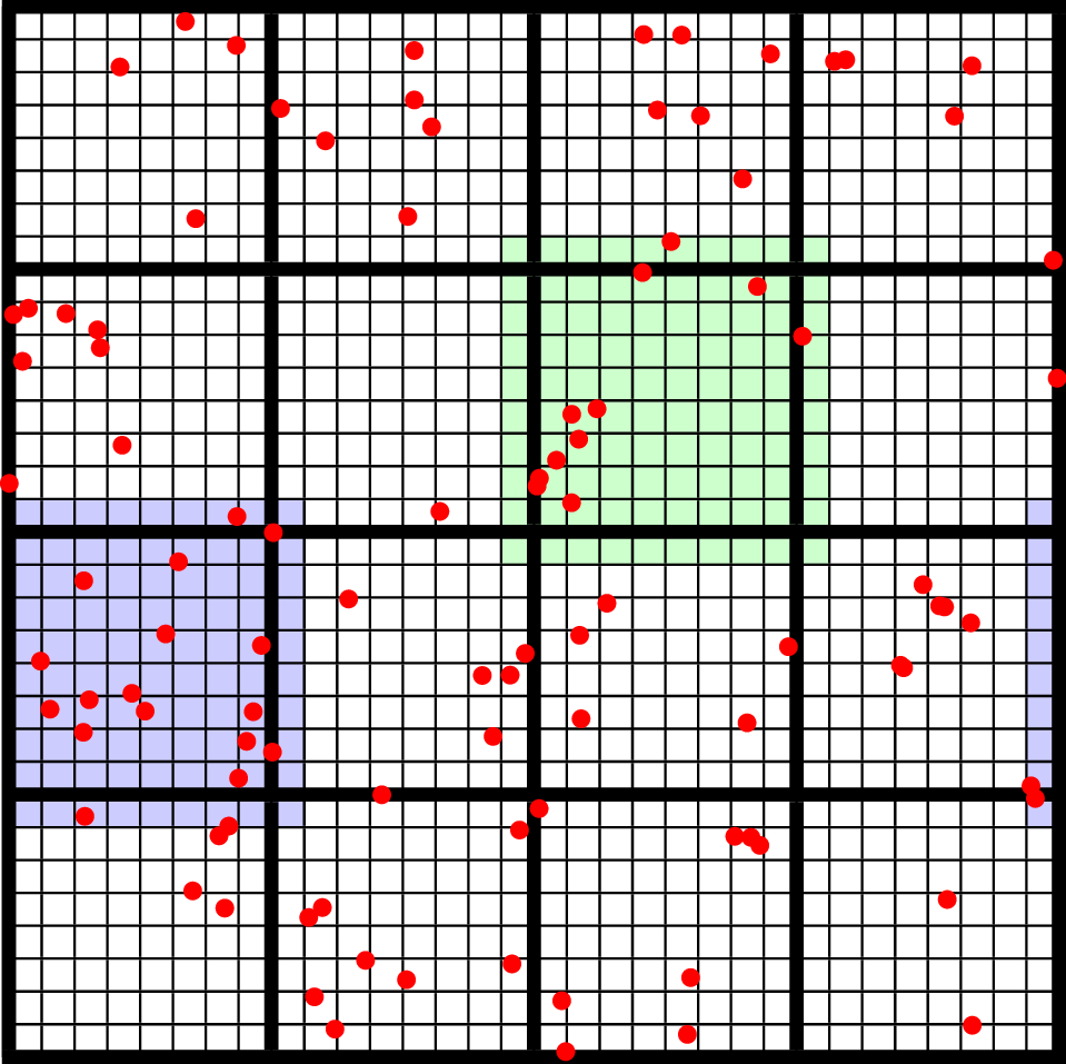
Fig. 9 : An illustration of filling neighbor particles for short-range force calculations. Here, we have a domain consisting of one \(32 \times 32\) grid, broken up into \(8 \times 8\) tiles. The number of ghost cells is taken to be \(1\). For the tile in green, particles on other tiles in the entire shaded region will copied and packed into the green tile’s neighbor buffer. These particles can then be included in the force calculation. If the domain is periodic, particles in the grown region for the blue tile that lie on the other side of the domain will also be copied, and their positions will modified so that a naive distance calculation between valid particles and neighbors will be correct.

For a ParticleContainer that does this neighbor finding, please see NeighborParticleContainer in amrex/Src/Particles/AMReX_NeighborParticleContainer.H. The NeighborParticleContainer has additional methods called fillNeighbors() and clearNeighbors() that fill the neighbors data structure with copies of the proper particles. A tutorial that uses these features is available at NeighborList. In this tutorial the function void MDParticleContainer:computeForces() computes the forces on a given tile via direct summation over the real and neighbor particles, as follows:

void MDParticleContainer::computeForces()
{
    BL_PROFILE("MDParticleContainer::computeForces");

    const int lev = 0;
    const Geometry& geom = Geom(lev);
    auto& plev  = GetParticles(lev);

    for(MFIter mfi = MakeMFIter(lev); mfi.isValid(); ++mfi)
    {
        int gid = mfi.index();
        int tid = mfi.LocalTileIndex();
        auto index = std::make_pair(gid, tid);

        auto& ptile = plev[index];
        auto& aos   = ptile.GetArrayOfStructs();
        const size_t np = aos.numParticles();

        auto nbor_data = m_neighbor_list[lev][index].data();
        ParticleType* pstruct = aos().dataPtr();

       // now we loop over the neighbor list and compute the forces
        AMREX_FOR_1D ( np, i,
        {
            ParticleType& p1 = pstruct[i];
            p1.rdata(PIdx::ax) = 0.0;
            p1.rdata(PIdx::ay) = 0.0;
            p1.rdata(PIdx::az) = 0.0;

            for (const auto& p2 : nbor_data.getNeighbors(i))
            {
                Real dx = p1.pos(0) - p2.pos(0);
                Real dy = p1.pos(1) - p2.pos(1);
                Real dz = p1.pos(2) - p2.pos(2);

                Real r2 = dx*dx + dy*dy + dz*dz;
                r2 = amrex::max(r2, Params::min_r*Params::min_r);

                if (r2 > Params::cutoff*Params::cutoff) return;

                Real r = sqrt(r2);

                Real coef = (1.0 - Params::cutoff / r) / r2;
                p1.rdata(PIdx::ax) += coef * dx;
                p1.rdata(PIdx::ay) += coef * dy;
                p1.rdata(PIdx::az) += coef * dz;
            }
        });
    }
}

Doing a direct \(N^2\) summation over the particles on a tile is avoided by binning the particles by cell and building a neighbor list. The data structure used to represent the neighbor lists is illustrated in Fig. 10.

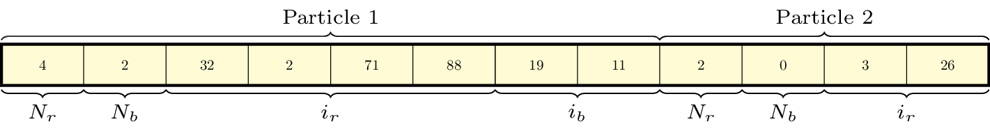
Fig. 10 : An illustration of the neighbor list data structure used by AMReX. The list for each tile is represented by an array of integers. The first number in the array is the number of real (i.e., not in the neighbor buffers) collision partners for the first particle on this tile, while the second is the number of collision partners from nearby tiles in the neighbor buffer. Based on the number of collision partners, the next several entries are the indices of the collision partners in the real and neighbor particle arrays, respectively. This pattern continues for all the particles on this tile.

This array can then be used to compute the forces on all the particles in one scan. Users can define their own NeighborParticleContainer subclasses that have their own collision criteria by overloading the virtual check_pair function.

Particle IO

AMReX provides routines for writing particle data to disk for analysis, visualization, and for checkpoint / restart. The most important methods are the WritePlotFile, Checkpoint, and Restart methods of ParticleContainer, which all use a parallel-aware binary file format for reading and writing particle data on a grid-by-grid basis. These methods are designed to complement the functions in AMReX_PlotFileUtil.H for performing mesh data IO. For example:

WriteMultiLevelPlotfile("plt00000", output_levs, GetVecOfConstPtrs(output),
                        varnames, geom, 0.0, level_steps, outputRR);
pc.Checkpoint("plt00000", "particle0");

will create a plot file called “plt00000” and write the mesh data in output to it, and then write the particle data in a subdirectory called “particle0”. There is also the WriteAsciiFile method, which writes the particles in a human-readable text format. This is mainly useful for testing and debugging.

The binary file format is readable by either yt or Paraview. See the chapter on Visualization for more information on visualizing AMReX datasets, including those with particles.

Inputs parameters

There are several runtime parameters users can set in their inputs files that control the behavior of the AMReX particle classes. These are summarized below. They should be preceded by “particles” in your inputs deck.

The first set of parameters concerns the tiling capability of the ParticleContainer. If you are seeing poor performance with OpenMP, the first thing to look at is whether there are enough tiles available for each thread to work on.

	Description	Type	Default
do_tiling	Whether to use tiling for particles. Should be on when using OpenMP, and off when running on GPUs.	Bool	false
tile_size	If tiling is on, the maximum tile_size to in each direction	Ints	1024000,8,8

The next set concerns runtime parameters that control the particle IO. Parallel file systems tend not to like it when too many MPI tasks touch the disk at once. Additionally, performance can degrade if all MPI tasks try writing to the same file, or if too many small files are created. In general, the “correct” values of these parameters will depend on the size of your problem (i.e., number of boxes, number of MPI tasks), as well as the system you are using. If you are experiencing problems with particle IO, you could try varying some / all of these parameters.

	Description	Type	Default
particles_nfiles	How many files to use when writing particle data to plt directories	Int	1024
nreaders	How many MPI tasks to use as readers when initializing particles from binary files.	Ints	64
nparts_per_read	How many particles each task should read from said files before calling Redistribute	Ints	100000
datadigits_read	This for backwards compatibility, don’t use unless you need to read and old (pre mid 2017) AMReX dataset.	Int	5
use_prepost	This is an optimization for large particle datasets that groups MPI calls needed during the IO together. Try it seeing poor IO speeds on large problems.	Bool	false

The following runtime parameters affect the behavior of virtual particles in Nyx.

	Description	Type	Default
aggregation_type	How to create virtual particles from finer levels. The options are: “None” - don’t do any aggregation. “Cell” - when creating virtuals, combine all particles that are in the same cell.	String	“None”
aggregation_buffer	If aggregation on, the number of cells around the coarse/fine boundary in which no aggregation should be performed.	Int	2

[1]

Particles default to double precision for their real data. To use single precision, compile your code with USE_SINGLE_PRECISION_PARTICLES=TRUE.

[2]

Note that for the extra particle components, which component refers to which variable is an application-specific convention - the particles have 4 extra real comps, but which one is “mass” is up to the user. We suggest using an enum to keep these indices straight; please see amrex-tutorials/ExampleCodes/Particles/ElectrostaticPIC/ElectrosticParticleContainer.H for an example of this.