Initializing the Geometric Database
In AMReX, geometric information is stored in a distributed database class that must be initialized at the start of the calculation. The procedure is as follows:
Define an implicit function of position which describes the surface of the embedded object. Specifically, the function class must have a public member function that takes a position and returns a negative value if that position is inside the fluid, a positive value in the body, and identically zero at the embedded boundary.
Real operator() (const Array<Real,AMREX_SPACEDIM>& p) const;
Make a
EB2::GeometryShopobject using the implicit function.Build an
EB2::IndexSpacewith theEB2::GeometryShopobject and aGeometryobject that contains the information about the domain and the mesh.
Here is a simple example of initializing the database for an embedded sphere.
Real radius = 0.5;
Array<Real,AMREX_SPACEDIM> center{0., 0., 0.}; //Center of the sphere
bool inside = false;  // Is the fluid inside the sphere?
EB2::SphereIF sphere(radius, center, inside);

auto shop = EB2::makeShop(sphere);

Geometry geom(...);
EB2::Build(shop, geom, 0, 0);
Alternatively, the EB information can be initialized from an STL file
specified by a ParmParse parameter eb2.stl_file. (This also requires setting eb2.geom_type = stl.) The
initialization is done by calling
EB2::Build (const Geometry& geom,
            int required_coarsening_level,
            int max_coarsening_level,
            int ngrow = 4,
            bool build_coarse_level_by_coarsening = true);
Additionally, one can use eb2.stl_scale, eb2.stl_center and
eb2.stl_reverse_normal to scale, translate and reverse the object,
respectively.
Implicit Function
In amrex/Src/EB/, there are a number of predefined implicit function classes
for basic shapes. One can use these directly or as templates for their own
classes.
AllRegularIF: No embedded boundaries at all.BoxIF: Box.CylinderIF: Cylinder.EllipsoidIF: Ellipsoid.PlaneIF: Half-space plane.SphereIF: Sphere.
AMReX also provides a number of transformation operations to apply to an object.
makeComplement: Complement of an object. E.g., a sphere with fluid on the outside becomes a sphere with fluid inside.makeIntersection: Intersection of two or more objects.makeUnion: Union of two or more objects.Translate: Translates an object.scale: Scales an object.rotate: Rotates an object.lathe: Creates a surface of revolution by rotating a 2D object around an axis.
Here are some examples of using these functions.
EB2::SphereIF sphere1(...);
EB2::SphereIF sphere2(...);
EB2::BoxIF box(...);
EB2::CylinderIF cylinder(...);
EB2::PlaneIF plane(...);

// union of two spheres
auto twospheres = EB2::makeUnion(sphere1, sphere2);

// intersection of a rotated box, a plane and the union of two spheres
auto box_plane = EB2::makeIntersection(amrex::rotate(box,...),
                                       plane,
                                       twospheres);

// scale a cylinder by a factor of 2 in x and y directions, and 3 in z-direction.
auto scylinder = EB2::scale(cylinder, {2., 2., 3.});
EB2::GeometryShop
Given an implicit function object, say f, we can make a
GeometryShop object with
auto shop = EB2::makeShop(f);
EB2::IndexSpace
We build EB2::IndexSpace with one of several functions depending
on the application needs.
Standard Build with Automatic Coarsening
template <typename G>
void EB2::Build (const G& gshop, const Geometry& geom,
                 int required_coarsening_level,
                 int max_coarsening_level,
                 int ngrow = 4,
                 bool build_coarse_level_by_coarsening = true,
                 bool extend_domain_face = ExtendDomainFace(),
                 int num_coarsen_opt = NumCoarsenOpt());
Here the template parameter is a EB2::GeometryShop. Geometry (see
section RealBox and Geometry) describes the rectangular problem domain and the
mesh on the finest AMR level. Coarse level EB data is generated from coarsening
the original fine data. The int required_coarsening_level parameter
specifies the number of coarsening levels required. This is usually set to
\(N-1\), where \(N\) is the total number of AMR levels. The int
max_coarsening_levels parameter specifies the number of coarsening levels AMReX
should try to have. This is usually set to a big number, say 20 if multigrid
solvers are used. This essentially tells the build to coarsen as much as it can.
If there are no multigrid solvers, the parameter should be set to the same as
required_coarsening_level. It should be noted that coarsening could
create multi-valued cells even if the fine level does not have any multi-valued
cells. This occurs when the embedded boundary cuts a cell in such a way that
there is fluid on multiple sides of the boundary within that cell. Because
multi-valued cells are not supported, it will cause a runtime error if the
required coarsening level generates multi-valued cells. The optional int
ngrow parameter specifies the number of ghost cells outside the domain on
required levels. For levels coarser than the required level, no EB data are
generated for ghost cells outside the domain.
Build with Explicit Multi-Level Geometry
For applications requiring explicit control over the geometry at each AMR level:
template <typename G>
void EB2::Build (const G& gshop, Vector<Geometry> geom,
int ngrow = 4,
bool extend_domain_face = ExtendDomainFace(),
int num_coarsen_opt = NumCoarsenOpt());
This version takes a Vector<Geometry> where each element corresponds to
the geometry of a specific AMR level. The vector can be unordered, as it will be
sorted based on numPts.
Unlike the standard Build function, coarse level EB data is generated
directly from the provided geometries rather than through automatic coarsening.
This is useful when coarse level domains are not simple coarsenings of the fine
level, or when you need precise control over the domain and mesh spacing at each
level.
Build from STL File
As mentioned earlier, the EB information can alternatively be initialized from an STL file using:
void EB2::Build (const Geometry& geom,
                 int required_coarsening_level,
                 int max_coarsening_level,
                 int ngrow = 4,
                 bool build_coarse_level_by_coarsening = true,
                 bool extend_domain_face = ExtendDomainFace(),
                 int num_coarsen_opt = NumCoarsenOpt());
This requires setting ParmParse parameters eb2.geom_type = stl and
eb2.stl_file to specify the STL file path.
Managing IndexSpace Objects
Regardless of which Build variant is used, the newly built
EB2::IndexSpace is pushed onto a stack. Static function
EB2::IndexSpace::top() returns a const & to the new
EB2::IndexSpace object. We usually only need to build one
EB2::IndexSpace object. However, if your application needs multiple
EB2::IndexSpace objects, you can save the pointers for later use. For
simplicity, we assume there is only one EB2::IndexSpace object for the rest of
this chapter.
EBFArrayBoxFactory
After the EB database is initialized, the next object we build is
EBFArrayBoxFactory. This object provides access to the EB database in the
format of basic AMReX objects such as BaseFab, FArrayBox,
FabArray, and MultiFab. We can construct it with
EBFArrayBoxFactory (const Geometry& a_geom,
                    const BoxArray& a_ba,
                    const DistributionMapping& a_dm,
                    const Vector<int>& a_ngrow,
                    EBSupport a_support);
or
std::unique_ptr<EBFArrayBoxFactory>
makeEBFabFactory (const Geometry& a_geom,
                  const BoxArray& a_ba,
                  const DistributionMapping& a_dm,
                  const Vector<int>& a_ngrow,
                  EBSupport a_support);
Argument Vector<int> const& a_ngrow specifies the number of
ghost cells we need for EB data at various EBSupport levels,
and argument EBSupport a_support specifies the level of support
needed.
EBSupport::basic: basic flags for cell typesEBSupport::volume: basic plus volume fraction and centroidEBSupport::full: volume plus area fraction, boundary centroid and face centroid
EBFArrayBoxFactory is derived from FabFactory<FArrayBox>.
MultiFab constructors have an optional argument const
FabFactory<FArrayBox>&. We can use EBFArrayBoxFactory to
build MultiFabs that carry EB data. The member function of
FabArray
const FabFactory<FAB>& Factory () const;
can then be used to return a reference to the EBFArrayBoxFactory used for
building the MultiFab. Using dynamic_cast, we can test whether a
MultiFab is built with an EBFArrayBoxFactory.
auto factory = dynamic_cast<EBFArrayBoxFactory const*>(&(mf.Factory()));
if (factory) {
    // this is EBFArrayBoxFactory
} else {
    // regular FabFactory<FArrayBox>
}
Embedded Boundary Data
Through member functions of EBFArrayBoxFactory, we have access to the
following data:
// see section on EBCellFlagFab
const FabArray<EBCellFlagFab>& getMultiEBCellFlagFab () const;

// volume fraction
const MultiFab& getVolFrac () const;

// volume centroid
const MultiCutFab& getCentroid () const;

// embedded boundary centroid
const MultiCutFab& getBndryCent () const;

// embedded boundary normal direction
const MultiCutFab& getBndryNormal () const;

// embedded boundary surface area
const MultiCutFab& getBndryArea () const;

// area fractions
Array<const MultiCutFab*,AMREX_SPACEDIM> getAreaFrac () const;

// face centroid
Array<const MultiCutFab*,AMREX_SPACEDIM> getFaceCent () const;
Volume fraction is stored in a single-component
MultiFab. Data are in the range of \([0,1]\) with zero representing covered cells and one for regular cells.Volume centroid (also called cell centroid) is in a
MultiCutFabwithAMREX_SPACEDIMcomponents. Each component of the data is in the range \([-0.5,0.5]\), based on each cell’s local coordinates with respect to the regular cell’s center.Boundary centroid is also in a
MultiCutFabwithAMREX_SPACEDIMcomponents. Each component of the data is in the range \([-0.5,0.5]\), based on each cell’s local coordinates with respect to the regular cell’s center.Boundary normal is in a
MultiCutFabwithAMREX_SPACEDIMcomponents representing the unit vector pointing toward the covered part.Boundary area is in a
MultiCutFabwith a single component representing the dimensionless boundary area. When the cell is isotropic (i.e., \(\Delta x = \Delta y = \Delta z\)), it’s trivial to convert it to physical units. If the cell size is anisotropic, the conversion requires multiplying by a factor of \(\sqrt{(n_x \Delta y \Delta z)^2 + (n_y \Delta x \Delta z)^2 + (n_z \Delta x \Delta y)^2}\), where \(n\) is the boundary normal vector.Area fractions are returned in an
ArrayofMultiCutFabpointers. For each direction, the area fraction is for the face in that direction. Data are in the range of \([0,1]\) with zero representing a covered face and one an un-cut face.Face centroids are returned in an
ArrayofMultiCutFabpointers. There are two components for each direction, and the ordering is always the same as the original ordering of the coordinates. For example, for \(y\) face, the component 0 is for \(x\) coordinate and 1 for \(z\). The coordinates are in each face’s local frame normalized to the range of \([-0.5,0.5]\).
Embedded Boundary Data Structures
A MultiCutFab is very similar to a MultiFab. Its data can be
accessed with subscript operator
const CutFab& operator[] (const MFIter& mfi) const;
Here CutFab is derived from FArrayBox and can be passed to Fortran
just like FArrayBox. The difference between MultiCutFab and
MultiFab is that to save memory MultiCutFab only has data on boxes
that contain cut cells. It is an error to call operator[] if that box
does not have cut cells. Thus the call must be in a if test block (see
section EBCellFlagFab).
EBCellFlagFab
EBCellFlagFab contains information on cell types. We can use
it to determine if a box contains cut cells.
auto const& flags = factory->getMultiEBCellFlagFab();
MultiCutFab const& centroid = factory->getCentroid();

for (MFIter mfi ...) {
    const Box& bx = mfi.tilebox();
    FabType t = flags[mfi].getType(bx);
    if (FabType::regular == t) {
        // This box is regular
    } else if (FabType::covered == t) {
        // This box is covered
    } else if (FabType::singlevalued == t) {
        // This box has cut cells
        // Getting cutfab is safe
        const auto& centroid_fab = centroid[mfi];
    }
}
EBCellFlagFab is derived from BaseFab. Its data are stored in an
array of 32-bit integers, and can be used in C++ or passed to Fortran just like
an IArrayBox (section BaseFab, FArrayBox, IArrayBox, and Array4). AMReX provides a Fortran
module called amrex_ebcellflag_module. This module contains procedures for
testing cell types and getting neighbor information. For example
use amrex_ebcellflag_module, only : is_regular_cell, is_single_valued_cell, is_covered_cell

integer, intent(in) :: flags(...)

integer :: i,j,k

do k = ...
    do j = ...
        do i = ...
            if (is_covered_cell(flags(i,j,k))) then
                ! this is a completely covered cell
            else if (is_regular_cell(flags(i,j,k))) then
                ! this is a regular cell
            else if (is_single_valued_cell(flags(i,j,k))) then
                ! this is a cut cell
            end if
        end do
    end do
end do
Small Cell Problem and Redistribution
First, we review finite volume discretizations with embedded boundaries as used by AMReX-based applications. Then we illustrate the small cell problem.
Finite Volume Discretizations
Consider a system of PDEs to advance a conserved quantity \(U\) with fluxes \(F\):
A conservative, finite volume discretization starts with the divergence theorem
In an embedded boundary cell, the “conservative divergence” is discretized (as \(D^c(F)\)) as follows
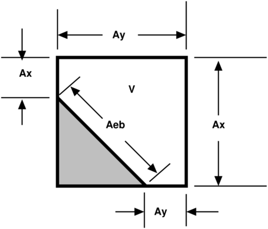
Geometry is discretely represented by volumes (\(V = \kappa h^d\)) and apertures (\(A= \alpha h^{d-1}\)), where \(h\) is the (uniform) mesh spacing at that AMR level, \(\kappa\) is the volume fraction and \(\alpha\) are the area fractions. Without multivalued cells the volume fractions, area fractions and cell and face centroids (see Table 11) are the only geometric information needed to compute second-order fluxes centered at the face centroids, and to infer the connectivity of the cells. Cells are connected if adjacent on the Cartesian mesh, and only via coordinate-aligned faces on the mesh. If an aperture, \(\alpha = 0\), between two cells, they are not directly connected to each other.
|
|
A typical two-dimensional uniform cell that is
cut by the embedded boundary. The grey area
represents the region excluded from the
calculation. The portion of the cell faces
faces (labelled with A) through which fluxes
flow are the “uncovered” regions of the full
cell faces. The volume (labelled V) is the
uncovered region of the interior.
|
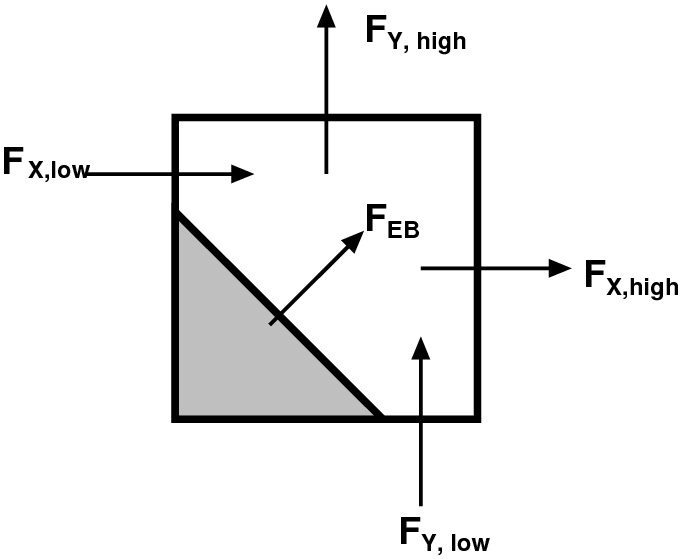
Fluxes in a cut cell.
|
Small Cells and Stability
In the context of time-explicit advance methods for, say hyperbolic conservation laws, a naive discretization in time of (2) using (3),
would have a time step constraint \(\delta t \sim h \kappa^{1/D}/V_m\), which goes to zero as the size of the smallest volume fraction \(\kappa\) in the calculation. Since EB volume fractions can be arbitrarily small, this presents an unacceptable constraint. This is the so-called “small cell problem,” and AMReX-based applications address it with redistribution methods.
Flux Redistribution
Consider a conservative update in the form:
For each valid cell in the domain, compute the conservative divergence, \((\nabla \cdot F)^c\) , of the convective fluxes, \(F\)
Here \(N_f\) is the number of faces of cell \(i\), \(\vec{n}_f\) and \(A_f\) are the unit normal and area of the \(f\) -th face respectively, and \(\mathcal{V}_i\) is the volume of cell \(i\) given by
where \(\mathcal{K}_i\) is the volume fraction of cell \(i\) .
Now, a conservative update can be written as
For each cell cut by the EB geometry, compute the non-conservative update, \(\nabla \cdot {F}^{nc}\) ,
where \(N(i)\) is the index set of cell \(i\) and its neighbors.
For each cell cut by the EB geometry, compute the convective update \(\nabla \cdot{F}^{EB}\) as follows:
For each cell cut by the EB geometry, redistribute its mass loss, \(\delta M_i\) , to its neighbors:
where the mass loss in cell \(i\), \(\delta M_i\), is given by
and the weights, \(w_{ij}\) , are
Note that \(\nabla \cdot{F}_i^{EB}\) gives an update for \(\rho \phi\) ; i.e.,
Typically, the redistribution neighborhood for each cell is one that can be reached via a monotonic path in each coordinate direction of unit length (see, e.g., Fig. 12)
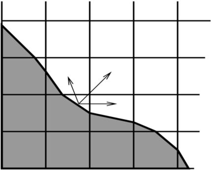
Fig. 12 Redistribution illustration. Excess update distributed to neighbor cells.
State Redistribution
For state redistribution, we implement the weighted state redistribution algorithm as described in Guiliani et al (2021), which is available on arXiv. This is an extension of the original state redistribution algorithm of Berger and Guiliani (2020).
Linear Solvers
Linear solvers for the canonical form (equation (1)) have been discussed in Chapter Linear Solvers.
AMReX supports multi-level 1) cell-centered solvers with homogeneous Neumann, homogeneous Dirichlet, or inhomogeneous Dirichlet boundary conditions on the EB faces, and 2) nodal solvers with homogeneous Neumann boundary conditions, or inflow velocity conditions on the EB faces.
To use a cell-centered solver with EB, one builds a linear operator
MLEBABecLap with EBFArrayBoxFactory (instead of a MLABecLaplacian)
MLEBABecLap (const Vector<Geometry>& a_geom,
             const Vector<BoxArray>& a_grids,
             const Vector<DistributionMapping>& a_dmap,
             const LPInfo& a_info,
             const Vector<EBFArrayBoxFactory const*>& a_factory);
The usage of this EB-specific class is essentially the same as
MLABecLaplacian.
The default boundary condition on EB faces is homogeneous Neumann.
To set homogeneous Dirichlet boundary conditions, call
ml_ebabeclap->setEBHomogDirichlet(lev, coeff);
where coeff can be a real number (i.e. the value is the same at every cell) or is the MultiFab holding the coefficient of the gradient at each cell with an EB face.
To set inhomogeneous Dirichlet boundary conditions, call
ml_ebabeclap->setEBDirichlet(lev, phi_on_eb, coeff);
where phi_on_eb is the MultiFab holding the Dirichlet values in every cut cell, and coeff again is a real number (i.e. the value is the same at every cell) or a MultiFab holding the coefficient of the gradient at each cell with an EB face.
Currently there are options to define the face-based coefficients on face centers vs face centroids, and to interpret the solution variable as being defined on cell centers vs cell centroids.
The default is for the solution variable to be defined at cell centers; to tell the solver to interpret the solution variable as living at cell centroids, you must set
ml_ebabeclap->setPhiOnCentroid();
The default is for the face-based coefficients to be defined at face centers; to tell the solver that the face-based coefficients should be interpreted as living at face centroids, modify the setBCoeffs command to be
ml_ebabeclap->setBCoeffs(lev, beta, MLMG::Location::FaceCentroid);
Tutorials
EB/CNS is an AMR code for solving compressible Navier-Stokes equations with the embedded boundary approach.
EB/Poisson is a single-level code that is a proxy for solving the electrostatic Poisson equation for a grounded sphere with a point charge inside.
EB/MacProj is a single-level code that computes a divergence-free flow field around a sphere. A MAC projection is performed on an initial velocity field of (1,0,0).