MLMG and Linear Operator Classes

Multi-Level Multi-Grid or MLMG is a class for solving the linear system using the geometric multigrid method. The constructor of MLMG takes the reference to MLLinOp, an abstract base class of various linear operator classes, MLABecLaplacian, MLPoisson, MLNodeLaplacian, etc. We choose the type of linear operator class according to the type the linear system to solve.

MLABecLaplacian for cell-centered canonical form (equation (1)).
MLPoisson for cell-centered constant coefficient Poisson’s equation \(\nabla^2 \phi = f\).
MLNodeLaplacian for nodal variable coefficient Poisson’s equation \(\nabla \cdot (\sigma \nabla \phi) = f\).

The constructors of these linear operator classes are in the form like below

MLABecLaplacian (const Vector<Geometry>& a_geom,
                 const Vector<BoxArray>& a_grids,
                 const Vector<DistributionMapping>& a_dmap,
                 const LPInfo& a_info = LPInfo(),
                 const Vector<FabFactory<FArrayBox> const*>& a_factory = {},
                 const int a_ncomp = 1);

It takes Vectors of Geometry, BoxArray and DistributionMapping. The arguments are Vectors because MLMG can do multi-level composite solves. If you are using it for single-level, you can do

// Given Geometry geom, BoxArray grids, and DistributionMapping dmap on single level
MLABecLaplacian mlabeclaplacian({geom}, {grids}, {dmap});

to let the compiler construct Vectors for you. Recall that the classes Vector, Geometry, BoxArray, and DistributionMapping are defined in chapter Basics. There are two new classes that are optional parameters. LPInfo is a class for passing parameters. FabFactory is used in problems with embedded boundaries (chapter Embedded Boundaries).

After the linear operator is built, we need to set up boundary conditions. This will be discussed later in section Boundary Conditions.

Coefficients

Next, we consider the coefficients for equation (1). For MLPoisson, there are no coefficients to set so nothing needs to be done. For MLABecLaplacian, we need to call member functions setScalars, setACoeffs, and setBCoeffs. The setScalars function sets the scalar constants \(A\) and \(B\)

void setScalars (Real a, Real b) noexcept;

For the general case where \(\alpha\) and \(\beta\) are scalar fields, we use

void setACoeffs (int amrlev, const MultiFab& alpha);
void setBCoeffs (int amrlev, const Array<MultiFab const*,AMREX_SPACEDIM>& beta);

For the case where \(\alpha\) and/or \(\beta\) are scalar constants, there is the option to use

void setACoeffs (int amrlev, Real alpha);
void setBCoeffs (int amrlev, Real beta);
void setBCoeffs (int amrlev, Vector<Real> const& beta);

Note, however, that the solver behavior is the same regardless of which functions you use to set the coefficients. These functions solely copy the constant value(s) to a MultiFab internal to MLMG and so no appreciable efficiency gains can be expected.

For MLNodeLaplacian, one can set a variable sigma with the member function

void setSigma (int amrlev, const MultiFab& a_sigma);

or a constant sigma during declaration or definition

MLNodeLaplacian (const Vector<Geometry>& a_geom,
                 const Vector<BoxArray>& a_grids,
                 const Vector<DistributionMapping>& a_dmap,
                 const LPInfo& a_info = LPInfo(),
                 const Vector<FabFactory<FArrayBox> const*>& a_factory = {},
                 Real  a_const_sigma = Real(0.0));

void define (const Vector<Geometry>& a_geom,
             const Vector<BoxArray>& a_grids,
             const Vector<DistributionMapping>& a_dmap,
             const LPInfo& a_info = LPInfo(),
             const Vector<FabFactory<FArrayBox> const*>& a_factory = {},
             Real  a_const_sigma = Real(0.0));

Here, setting a constant sigma alters the internal behavior of the solver making it more efficient for this special case.

The int amrlev parameter should be zero for single-level solves. For multi-level solves, each level needs to be provided with alpha and beta, or sigma. For composite solves, amrlev 0 will mean the lowest level for the solver, which is not necessarily the lowest level in the AMR hierarchy. This is so solves can be done on different sections of the AMR hierarchy, e.g. on AMR levels 3 to 5.

After boundary conditions and coefficients are prescribed, the linear operator is ready for an MLMG object like below.

MLMG mlmg(mlabeclaplacian);

Optional parameters can be set (see section Parameters), and then we can use the MLMG member function

Real solve (const Vector<MultiFab*>& a_sol,
            const Vector<MultiFab const*>& a_rhs,
            Real a_tol_rel, Real a_tol_abs);

to solve the problem given an initial guess and a right-hand side. Zero is a perfectly fine initial guess. The two Reals in the argument list are the targeted relative and absolute error tolerances. The relative error tolerance is hard-coded to be at least \(10^{-16}\). Given the linear system \(Ax=b\), the solver will terminate when the max-norm of the residual (\(b-Ax\)) is less than std::max(a_tol_abs, a_tol_rel*max_norm) where max_norm is the max-norm of the rhs, \(b\), if the flag always_use_bnorm is set to True or if the rhs max-norm is greater than or equal to the max-norm error of the initial guess, otherwise max_norm is equal to the max-norm error of the initial guess. Set the absolute tolerance to zero if one does not have a good value for it. The return value of solve is the max-norm error.

After the solver returns successfully, if needed, we can call

void compResidual (const Vector<MultiFab*>& a_res,
                   const Vector<MultiFab*>& a_sol,
                   const Vector<MultiFab const*>& a_rhs);

to compute residual (i.e., \(f - L(\phi)\)) given the solution and the right-hand side. For cell-centered solvers, we can also call the following functions to compute gradient \(\nabla \phi\) and fluxes \(-\beta \nabla \phi\).

void getGradSolution (const Vector<Array<MultiFab*,AMREX_SPACEDIM> >& a_grad_sol);
void getFluxes       (const Vector<Array<MultiFab*,AMREX_SPACEDIM> >& a_fluxes);

Boundary Conditions

We now discuss how to set up boundary conditions for linear operators. In the following, physical domain boundaries refer to the boundaries of the physical domain, whereas coarse/fine boundaries refer to the boundaries between AMR levels. The following steps must be followed in the exact order.

1) For any type of solver, we first need to set physical domain boundary types via the MLLinOp member function

void setDomainBC (const Array<LinOpBCType,AMREX_SPACEDIM>& lobc,  // for lower ends
                  const Array<LinOpBCType,AMREX_SPACEDIM>& hibc); // for higher ends

The supported BC types at the physical domain boundaries are

LinOpBCType::Periodic for periodic boundary.
LinOpBCType::Dirichlet for Dirichlet boundary condition.
LinOpBCType::Neumann for homogeneous Neumann boundary condition.
LinOpBCType::inhomogNeumann for inhomogeneous Neumann boundary condition.
LinOpBCType::Robin for Robin boundary conditions, \(a\phi + b\frac{\partial\phi}{\partial n} = f\).
LinOpBCType::reflect_odd for reflection with sign changed.

2) Cell-centered solvers only: if we want to do a linear solve where the boundary conditions on the coarsest AMR level of the solve come from a coarser level (e.g. the base AMR level of the solve is > 0 and does not cover the entire domain), we must explicitly provide the coarser data. Boundary conditions from a coarser level are always Dirichlet.

Note that this step, if needed, must be performed before the step below. The MLLinOp member function for this step is

void setCoarseFineBC (const MultiFab* crse, int crse_ratio);

Here const MultiFab* crse contains the Dirichlet boundary values at the coarse resolution, and int crse_ratio (e.g., 2) is the refinement ratio between the coarsest solver level and the AMR level below it. The MultiFab crse does not need to have ghost cells itself. If the coarse grid bc’s for the solve are identically zero, nullptr can be passed instead of crse.

3) Cell-centered solvers only: before the solve one must always call the MLLinOp member function

virtual void setLevelBC (int amrlev, const MultiFab* levelbcdata,
                         const MultiFab* robinbc_a = nullptr,
                         const MultiFab* robinbc_b = nullptr,
                         const MultiFab* robinbc_f = nullptr) = 0;

If we want to supply an inhomogeneous Dirichlet or inhomogeneous Neumann boundary condition at the domain boundaries, we must supply those values in MultiFab* levelbcdata, which must have at least one ghost cell. Note that the argument amrlev is relative to the solve, not necessarily the full AMR hierarchy; amrlev = 0 refers to the coarsest level of the solve.

If the boundary condition is Dirichlet the ghost cells outside the domain boundary of levelbcdata must hold the value of the solution at the domain boundary; if the boundary condition is Neumann those ghost cells must hold the value of the gradient of the solution normal to the boundary (e.g. it would hold dphi/dx on both the low and high faces in the x-direction).

If the boundary conditions contain no inhomogeneous Dirichlet or Neumann boundaries, we can pass nullptr instead of a MultiFab.

We can use the solution array itself to hold these values; the values are copied to internal arrays and will not be over-written when the solution array itself is being updated by the solver. Note, however, that this call does not provide an initial guess for the solve.

It should be emphasized that the data in levelbcdata for Dirichlet or Neumann boundaries are assumed to be exactly on the face of the physical domain; storing these values in the ghost cell of a cell-centered array is a convenience of implementation.

For Robin boundary conditions, the ghost cells in MultiFab* robinbc_a, MultiFab* robinbc_b, and MultiFab* robinbc_f store the numerical values in the condition, \(a\phi + b\frac{\partial\phi}{\partial n} = f\).

Nodal solver provides the option to use an overset mask:

// omask is either 0 or 1. 1 means the node is an unknown. 0 means it's known.
void setOversetMask (int amrlev, const iMultiFab& a_dmask);

Note this is an integer (not bool) MultiFab, so the values must be only either 0 or 1.

Parameters

There are many parameters that can be set. Here we discuss some commonly used ones.

MLLinOp::setVerbose(int), MLMG::setVerbose(int) and MLMG:setBottomVerbose(int) control the verbosity of the linear operator, multigrid solver and the bottom solver, respectively.

The multigrid solver is an iterative solver. The maximal number of iterations can be changed with MLMG::setMaxIter(int). We can also do a fixed number of iterations with MLMG::setFixedIter(int). By default, V-cycle is used. We can use MLMG::setMaxFmgIter(int) to control how many full multigrid cycles can be done before switching to V-cycle.

LPInfo::setMaxCoarseningLevel(int) can be used to control the maximal number of multigrid levels. We usually should not call this function. However, we sometimes build the solver to simply apply the operator (e.g., \(L(\phi)\)) without needing to solve the system. We can do something as follows to avoid the cost of building coarsened operators for the multigrid.

MLABecLaplacian mlabeclap({geom}, {grids}, {dmap}, LPInfo().setMaxCoarseningLevel(0));
// set up BC
// set up coefficients
MLMG mlmg(mlabeclap);
// out = L(in)
mlmg.apply(out, in);  // here both in and out are const Vector<MultiFab*>&

At the bottom of the multigrid cycles, we use a bottom solver which may be different than the relaxation used at the other levels. The default bottom solver is the biconjugate gradient stabilized method, but can easily be changed with the MLMG member method

void setBottomSolver (BottomSolver s);

Available choices are

MLMG::BottomSolver::bicgstab: The default.
MLMG::BottomSolver::cg: The conjugate gradient method. The matrix must be symmetric.
MLMG::BottomSolver::smoother: Smoother such as Gauss-Seidel.
MLMG::BottomSolver::bicgcg: Start with bicgstab. Switch to cg if bicgstab fails. The matrix must be symmetric.
MLMG::BottomSolver::cgbicg: Start with cg. Switch to bicgstab if cg fails. The matrix must be symmetric.
MLMG::BottomSolver::hypre: One of the solvers available through hypre; see the section below on External Solvers
MLMG::BottomSolver::petsc: Currently for cell-centered only.
LPInfo::setAgglomeration(bool) (by default true) can be used continue to coarsen the multigrid by copying what would have been the bottom solver to a new MultiFab with a new BoxArray with fewer, larger grids, to allow for additional coarsening.
LPInfo::setConsolidation(bool) (by default true) can be used continue to transfer a multigrid problem to fewer MPI ranks. There are more setting such as LPInfo::setConsolidationGridSize(int), LPInfo::setConsolidationRatio(int), and LPInfo::setConsolidationStrategy(int), to give control over how this process works.

MLMG::setThrowException(bool) controls whether multigrid failure results in aborting (default) or throwing an exception, whereby control will return to the calling application. The application code must catch the exception:

try {
    mlmg.solve(...);
} catch (const MLMG::error& e) {
    Print()<<e.what()<<std::endl; //Prints description of error

    // Do something else...
}

Note that exceptions that are not caught are passed up the calling chain so that application codes using specialized solvers relying on MLMG can still catch the exception. For example, using AMReX-Hydro’s NodalProjector

try {
    nodal_projector.project(...);
} catch (const MLMG::error& e) {
    // Do something else...
}

Boundary Stencils for Cell-Centered Solvers

We have the option using the MLMG member method

void setMaxOrder (int maxorder);

to set the order of the cell-centered linear operator stencil at physical boundaries with Dirichlet boundary conditions and at coarse-fine boundaries. In both of these cases, the boundary value is not defined at the center of the ghost cell. The order determines the number of interior cells that are used in the extrapolation of the boundary value from the cell face to the center of the ghost cell, where the extrapolated value is then used in the regular stencil. For example, maxorder = 2 uses the boundary value and the first interior value to extrapolate to the ghost cell center; maxorder = 3 uses the boundary value and the first two interior values.

Curvilinear Coordinates

Some of the linear solvers support curvilinear coordinates including 1D spherical and 2d cylindrical \((r,z)\). In those cases, the divergence operator has extra metric terms. If one does not want the solver to include the metric terms because they have been handled in other ways, one can turn them off with a setter function. For the cell-centered linear solvers MLABecLaplacian and MLPoisson, one can call setMetricTerm(bool) with false on the LPInfo object passed to the constructor of linear operators. For the node-based MLNodeLaplacian, one can call setRZCorrection (bool) with false on the MLNodeLaplacian object.

MLABecLaplacian and MLPoisson support both spherical and cylindrical coordinates, while MLNodeLaplacian supports only cylindrical at this time. Note that to use cylindrical coordinates with MLNodeLaplacian, the application code must scale sigma by the radial coordinate before calling setSigma().

Embedded Boundaries

AMReX supports multi-level solvers for use with embedded boundaries. These include 1) cell-centered solvers with homogeneous Neumann, homogeneous Dirichlet, or inhomogeneous Dirichlet boundary conditions on the EB faces, and 2) nodal solvers with homogeneous Neumann boundary conditions, or inflow velocity conditions on the EB faces.

To use a cell-centered solver with EB, one builds a linear operator MLEBABecLap with EBFArrayBoxFactory (instead of a MLABecLaplacian)

MLEBABecLap (const Vector<Geometry>& a_geom,
             const Vector<BoxArray>& a_grids,
             const Vector<DistributionMapping>& a_dmap,
             const LPInfo& a_info,
             const Vector<EBFArrayBoxFactory const*>& a_factory);

The usage of this EB-specific class is essentially the same as MLABecLaplacian.

The default boundary condition on EB faces is homogeneous Neumann.

To set homogeneous Dirichlet boundary conditions, call

ml_ebabeclap->setEBHomogDirichlet(lev, coeff);

where coeff can be a real number (i.e. the value is the same at every cell) or a MultiFab holding the coefficient of the gradient at each cell with an EB face. In other words, coeff is \(\beta\) in the canonical form given in equation (1) located at the EB surface centroid.

To set inhomogeneous Dirichlet boundary conditions, call

ml_ebabeclap->setEBDirichlet(lev, phi_on_eb, coeff);

where phi_on_eb is the MultiFab holding the Dirichlet values in every cut cell, and coeff again is a real number or a MultiFab holding the coefficient of the gradient at each cell with an EB face, i.e. \(\beta\) in equation (1) located at the EB surface centroid.

Currently there are options to define the face-based coefficients on face centers vs face centroids, and to interpret the solution variable as being defined on cell centers vs cell centroids.

The default is for the solution variable to be defined at cell centers; to tell the solver to interpret the solution variable as living at cell centroids, you must set

ml_ebabeclap->setPhiOnCentroid();

The default is for the face-based coefficients to be defined at face centers; to tell the that the face-based coefficients should be interpreted as living at face centroids, modify the setBCoeffs command to be

ml_ebabeclap->setBCoeffs(lev, beta, MLMG::Location::FaceCentroid);

External Solvers

AMReX provides interfaces to the hypre preconditioners and solvers, including BoomerAMG, GMRES (all variants), PCG, and BICGStab as solvers, and BoomerAMG and Euclid as preconditioners. These can be called as as bottom solvers for both cell-centered and node-based problems.

If it is built with Hypre support, AMReX initializes Hypre by default in amrex::Initialize. If it is built with CUDA, AMReX will also set up Hypre to run on device by default. The user can choose to disable the Hypre initialization by AMReX with ParmParse parameter amrex.init_hypre=[0|1].

By default the AMReX linear solver code always tries to geometrically coarsen the problem as much as possible. However, as we have mentioned, we can call setMaxCoarseningLevel(0) on the LPInfo object passed to the constructor of a linear operator to disable the coarsening completely. In that case the bottom solver is solving the residual correction form of the original problem. To build Hypre, follow the next steps:

- git clone https://github.com/hypre-space/hypre.git
- cd hypre/src
- ./configure
    (if you want to build hypre with long long int, do ./configure --enable-bigint )
- make install
- Create an environment variable with the HYPRE directory --
    HYPRE_DIR=/hypre_path/hypre/src/hypre

To use hypre, one must include amrex/Src/Extern/HYPRE in the build system. For examples of using hypre, we refer the reader to ABecLaplacian or NodeTensorLap.

The following parameter should be set to True if the problem to be solved has a singular matrix. In this case, the solution is only defined to within a constant. Setting this parameter to True replaces one row in the matrix sent to hypre from AMReX by a row that sets the value at one cell to 0.

hypre.adjust_singular_matrix: Default is false.

The following parameters can be set in the inputs file to control the choice of preconditioner and smoother:

hypre.hypre_solver: Default is BoomerAMG.
hypre.hypre_preconditioner: Default is none; otherwise the type must be specified.
hypre.recompute_preconditioner: Default true. Option to recompute the preconditioner.
hypre.write_matrix_files: Default false. Option to write out matrix into text files.
hypre.overwrite_existing_matrix_files: Default false. Option to over-write existing matrix files.

The following parameters can be set in the inputs file to control the BoomerAMG solver specifically:

hypre.bamg_verbose: verbosity of BoomerAMG preconditioner. Default 0. See HYPRE_BoomerAMGSetPrintLevel
hypre.bamg_logging: Default 0. See HYPRE_BoomerAMGSetLogging
hypre.bamg_coarsen_type: Default 6. See HYPRE_BoomerAMGSetCoarsenType
hypre.bamg_cycle_type: Default 1. See HYPRE_BoomerAMGSetCycleType
hypre.bamg_relax_type: Default 6. See HYPRE_BoomerAMGSetRelaxType
hypre.bamg_relax_order: Default 1. See HYPRE_BoomerAMGSetRelaxOrder
hypre.bamg_num_sweeps: Default 2. See HYPRE_BoomerAMGSetNumSweeps
hypre.bamg_max_levels: Default 20. See HYPRE_BoomerAMGSetMaxLevels
hypre.bamg_strong_threshold: Default 0.25 for 2D, 0.57 for 3D. See HYPRE_BoomerAMGSetStrongThreshold
hypre.bamg_interp_type: Default 0. See HYPRE_BoomerAMGSetInterpType

The user is referred to the hypre Hypre Reference Manual for full details on the usage of the parameters described briefly above.

AMReX can also use PETSc as a bottom solver for cell-centered problems. To build PETSc, follow the next steps:

- git clone https://github.com/petsc/petsc.git
- cd petsc
- ./configure --prefix=build_dir
- Invoke the ``make all'' command given at the end of the previous command output
- Invoke the ``make install'' command given at the end of the previous command output
- Create an environment variable with the PETSC directory --
    PETSC_DIR=/petsc_path/petsc/build_dir

To use PETSc, one must include amrex/Src/Extern/PETSc in the build system. For an example of using PETSc, we refer the reader to the tutorial, ABecLaplacian.

Tensor Solve

Application codes that solve the Navier-Stokes equations need to evaluate the viscous term; solving for this term implicitly requires a multi-component solve with cross terms. Because this is a commonly used motif, we provide a tensor solve for cell-centered velocity components.

Consider a velocity field \(U = (u,v,w)\) with all components co-located on cell centers. The viscous term can be written in vector form as

\[\nabla \cdot (\eta \nabla U) + \nabla \cdot (\eta (\nabla U)^T ) + \nabla \cdot ( (\kappa - \frac{2}{3} \eta) (\nabla \cdot U) )\]

and in 3-d Cartesian component form as

\[ \begin{align}\begin{aligned}( (\eta u_x)_x + (\eta u_y)_y + (\eta u_z)_z ) + ( (\eta u_x)_x + (\eta v_x)_y + (\eta w_x)_z ) + ( (\kappa - \frac{2}{3} \eta) (u_x+v_y+w_z) )_x\\( (\eta v_x)_x + (\eta v_y)_y + (\eta v_z)_z ) + ( (\eta u_y)_x + (\eta v_y)_y + (\eta w_y)_z ) + ( (\kappa - \frac{2}{3} \eta) (u_x+v_y+w_z) )_y\\( (\eta w_x)_x + (\eta w_y)_y + (\eta w_z)_z ) + ( (\eta u_z)_x + (\eta v_z)_y + (\eta w_z)_z ) + ( (\kappa - \frac{2}{3} \eta) (u_x+v_y+w_z) )_z\end{aligned}\end{align} \]

Here \(\eta\) is the dynamic viscosity and \(\kappa\) is the bulk viscosity.

We evaluate the following terms from the above using the MLABecLaplacian and MLEBABecLaplacian operators;

\[ \begin{align}\begin{aligned}( (\frac{4}{3} \eta + \kappa) u_x)_x + ( \eta u_y)_y + (\eta u_z)_z\\ (\eta v_x)_x + ( (\frac{4}{3} \eta + \kappa) v_y)_y + (\eta v_z)_z\\ (\eta w_x)_x + ( \eta w_y)_y + ( (\frac{4}{3} \eta + \kappa) w_z)_z\end{aligned}\end{align} \]

the following cross-terms are evaluated separately using the MLTensorOp and MLEBTensorOp operators.

\[ \begin{align}\begin{aligned}( (\kappa - \frac{2}{3} \eta) (v_y + w_z) )_x + (\eta v_x)_y + (\eta w_x)_z\\(\eta u_y)_x + ( (\kappa - \frac{2}{3} \eta) (u_x + w_z) )_y + (\eta w_y)_z\\(\eta u_z)_x + (\eta v_z)_y - ( (\kappa - \frac{2}{3} \eta) (u_x + v_y) )_z\end{aligned}\end{align} \]

The code below is an example of how to set up the solver to compute the viscous term divtau explicitly:

Box domain(geom[0].Domain());

// Set BCs for Poisson solver in bc_lo, bc_hi
...

//
// First define the operator "ebtensorop"
// Note we call LPInfo().setMaxCoarseningLevel(0) because we are only applying the operator,
//      not doing an implicit solve
//
//       (alpha * a - beta * (del dot b grad)) sol
//
// LPInfo                       info;
MLEBTensorOp ebtensorop(geom, grids, dmap, LPInfo().setMaxCoarseningLevel(0),
                        amrex::GetVecOfConstPtrs(ebfactory));

// It is essential that we set MaxOrder of the solver to 2
// if we want to use the standard sol(i)-sol(i-1) approximation
// for the gradient at Dirichlet boundaries.
// The solver's default order is 3 and this uses three points for the
// gradient at a Dirichlet boundary.
ebtensorop.setMaxOrder(2);

// LinOpBCType Definitions are in amrex/Src/Boundary/AMReX_LO_BCTYPES.H
ebtensorop.setDomainBC ( {(LinOpBCType)bc_lo[0], (LinOpBCType)bc_lo[1], (LinOpBCType)bc_lo[2]},
                         {(LinOpBCType)bc_hi[0], (LinOpBCType)bc_hi[1], (LinOpBCType)bc_hi[2]} );

// Return div (eta grad)) phi
ebtensorop.setScalars(0.0, -1.0);

amrex::Vector<amrex::Array<std::unique_ptr<amrex::MultiFab>, AMREX_SPACEDIM>> b;
b.resize(max_level + 1);

// Compute the coefficients
for (int lev = 0; lev < nlev; lev++)
{
    // We average eta onto faces
    for(int dir = 0; dir < AMREX_SPACEDIM; dir++)
    {
        BoxArray edge_ba = grids[lev];
        edge_ba.surroundingNodes(dir);
        b[lev][dir] = std::make_unique<MultiFab>(edge_ba, dmap[lev], 1, nghost, MFInfo(), *ebfactory[lev]);
    }

    average_cellcenter_to_face( GetArrOfPtrs(b[lev]), *etan[lev], geom[lev] );

    b[lev][0] -> FillBoundary(geom[lev].periodicity());
    b[lev][1] -> FillBoundary(geom[lev].periodicity());
    b[lev][2] -> FillBoundary(geom[lev].periodicity());

    ebtensorop.setShearViscosity  (lev, GetArrOfConstPtrs(b[lev]));
    ebtensorop.setEBShearViscosity(lev, (*eta[lev]));

    ebtensorop.setLevelBC ( lev, GetVecOfConstPtrs(vel)[lev] );
}

MLMG solver(ebtensorop);

solver.apply(GetVecOfPtrs(divtau), GetVecOfPtrs(vel));

Multi-Component Operators

This section discusses solving linear systems in which the solution variable \(\mathbf{\phi}\) has multiple components. An example (implemented in the MultiComponent tutorial) might be:

\[D(\mathbf{\phi})_i = \sum_{i=1}^N \alpha_{ij} \nabla^2 \phi_j\]

(Note: only operators of the form \(D:\mathbb{R}^n\to\mathbb{R}^n\) are currently allowed.)

To implement a multi-component cell-based operator, inherit from the MLCellLinOp class. Override the getNComp function to return the number of components (N)that the operator will use. The solution and rhs fabs must also have at least one ghost node. Fapply, Fsmooth, Fflux must be implemented such that the solution and rhs fabs all have N components.
Implementing a multi-component node-based operator is slightly different. A MC nodal operator must specify that the reflux-free coarse/fine strategy is being used by the solver.
```
solver.setCFStrategy(MLMG::CFStrategy::ghostnodes);
```
The reflux-free method circumvents the need to implement a special reflux at the coarse-fine boundary. This is accomplished by using ghost nodes. Each AMR level must have 2 layers of ghost nodes. The second (outermost) layer of nodes is treated as constant by the relaxation, essentially acting as a Dirichlet boundary. The first layer of nodes is evolved using the relaxation, in the same manner as the rest of the solution. When the residual is restricted onto the coarse level (in reflux) this allows the residual at the coarse-fine boundary to be interpolated using the first layer of ghost nodes. Fig. 7 illustrates the how the coarse-fine update takes place.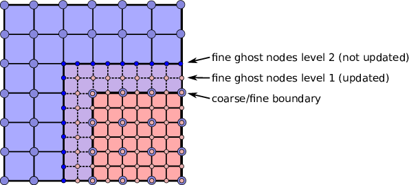

Fig. 7 Reflux-free coarse-fine boundary update. Level 2 ghost nodes (small dark blue) are interpolated from coarse boundary. Level 1 ghost nodes are updated during the relaxation along with all the other interior fine nodes. Coarse nodes (large blue) on the coarse/fine boundary are updated by restricting with interior nodes and the first level of ghost nodes. Coarse nodes underneath level 2 ghost nodes are not updated. The remaining coarse nodes are updates by restriction.

The MC nodal operator can inherit from the MCNodeLinOp class. Fapply, Fsmooth, and Fflux must update level 1 ghost nodes that are inside the domain. interpolation and restriction can be implemented as usual. reflux is a straightforward restriction from fine to coarse, using level 1 ghost nodes for restriction as described above.

See amrex-tutorials/ExampleCodes/LinearSolvers/MultiComponent for a complete working example.