CrayPat
The profiling suite available on Cray XC systems is Cray Performance
Measurement and Analysis Tools (“CrayPat”) [1]. Most CrayPat functionality is
supported for all compilers available in the Cray “programming environments”
(modules which begin “PrgEnv-“); however, a few features, chiefly the
“Reveal” tool, are supported only on applications compiled with Cray’s compiler
CCE [2] [3].
CrayPat supports both high-level profiling tools, as well as fine-grained performance analysis, such as reading hardware counters. The default behavior uses sampling to identify the most time-consuming functions in an application.
High-level application profiling
The simplest way to obtain a high-level overview of an application’s performance consists of the following steps:
Load the
perftools-basemodule, then theperftools-litemodule. (The modules will not work if loaded in the opposite order.)Compile the application with the Cray compiler wrappers
cc,CC, and/orftn. This works with any of the compilers available in thePrgEnv-modules. For example, on the Cori system at NERSC, one can use the Intel, GCC, or CCE compilers. No extra compiler flags are necessary in order for CrayPat to work. CrayPat instruments the application, so theperftools-modules must be loaded before one compiles the application.Run the application as normal. No special flags are required. Upon application completion, CrayPat will write a few files to the directory from which the application was launched. The profiling database is a single file with the
.ap2suffix.One can query the database in many different ways using the
pat_reportcommand on the.ap2file.pat_reportis available on login nodes, so the analysis need not be done on a compute node. Querying the database with no arguments topat_reportprints several different profiling reports to STDOUT, including a list of the most time-consuming regions in the application. The output of this command can be long, so it can be convenient to pipe the output to a pager or a file. A portion of the output frompat_report <file>.ap2is shown below:Table 1: Profile by Function Samp% | Samp | Imb. | Imb. | Group | | Samp | Samp% | Function | | | | PE=HIDE 100.0% | 5,235.5 | -- | -- | Total |----------------------------------------------------------------------------- | 50.2% | 2,628.5 | -- | -- | USER ||---------------------------------------------------------------------------- || 7.3% | 383.0 | 15.0 | 5.0% | eos_module_mp_iterate_ne_ || 5.7% | 300.8 | 138.2 | 42.0% | amrex_deposit_cic || 5.1% | 265.2 | 79.8 | 30.8% | update_dm_particles || 2.8% | 147.2 | 5.8 | 5.0% | fort_fab_setval || 2.6% | 137.2 | 48.8 | 34.9% | amrex::ParticleContainer<>::Where || 2.6% | 137.0 | 11.0 | 9.9% | ppm_module_mp_ppm_type1_ || 2.5% | 133.0 | 24.0 | 20.4% | eos_module_mp_nyx_eos_t_given_re_ || 2.1% | 107.8 | 33.2 | 31.4% | amrex::ParticleContainer<>::IncrementWithTotal || 1.7% | 89.2 | 19.8 | 24.2% | f_rhs_ || 1.4% | 74.0 | 7.0 | 11.5% | riemannus_ || 1.1% | 56.0 | 2.0 | 4.6% | amrex::VisMF::Write || 1.0% | 50.5 | 1.5 | 3.8% | amrex::VisMF::Header::CalculateMinMax ||============================================================================ | 28.1% | 1,471.0 | -- | -- | ETC ||---------------------------------------------------------------------------- || 7.4% | 388.8 | 10.2 | 3.4% | __intel_mic_avx512f_memcpy || 6.9% | 362.5 | 45.5 | 14.9% | CVode || 3.1% | 164.5 | 8.5 | 6.6% | __libm_log10_l9 || 2.9% | 149.8 | 29.2 | 21.8% | _INTERNAL_25_______src_kmp_barrier_cpp_5de9139b::__kmp_hyper_barrier_gather ||============================================================================ | 16.8% | 879.8 | -- | -- | MPI ||---------------------------------------------------------------------------- || 5.1% | 266.0 | 123.0 | 42.2% | MPI_Allreduce || 4.2% | 218.2 | 104.8 | 43.2% | MPI_Waitall || 2.9% | 151.8 | 78.2 | 45.4% | MPI_Bcast || 2.6% | 135.0 | 98.0 | 56.1% | MPI_Barrier || 2.0% | 105.8 | 5.2 | 6.3% | MPI_Recv ||============================================================================ | 1.9% | 98.2 | -- | -- | IO ||---------------------------------------------------------------------------- || 1.8% | 93.8 | 6.2 | 8.3% | read ||============================================================================
IPM - Cross-Platform Integrated Performance Monitoring
IPM provides portable profiling capabilities across HPC platforms, including support on selected Cray and IBM machines (cori and (TODO: verify it works on) summit). Running an IPM instrumented binary generates a summary of number of calls and time spent on MPI communication library functions. In addition, hardware performance counters can also be collected through PAPI.
Detailed instructions can be found at [4] and [5].
Building with IPM on Cori
Steps:
Run module load ipm.
Build code as normal with make.
Re-run the link command (e.g. cut-and-paste) with
$IPMadded to the end of the line.
Running with IPM on Cori
Set environment variables:
export IPM_REPORT=full IPM_LOG=full IPM_LOGDIR= <dir>Results will be printed to stdout, and an XML file will be generated in the directory specified by
IPM_LOGDIR.Post-process the XML with
ipm_parse -html <xmlfile>, which produces a directory with HTML.
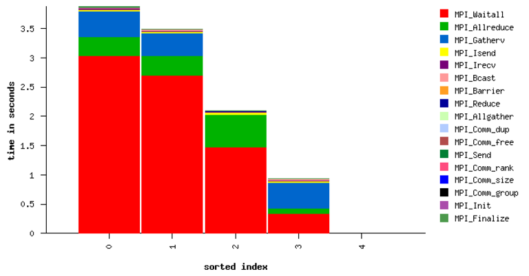
Summary MPI Profile
Example MPI profile output:
##IPMv2.0.5########################################################
#
# command   : /global/cscratch1/sd/cchan2/projects/lbl/BoxLib/Tests/LinearSolvers/C_CellMG/./main3d.intel.MPI.OMP.ex.ipm inputs.3d.25600
# start     : Tue Aug 15 17:34:23 2017   host      : nid11311
# stop      : Tue Aug 15 17:34:35 2017   wallclock : 11.54
# mpi_tasks : 128 on 32 nodes            %comm     : 32.51
# mem [GB]  : 126.47                     gflop/sec : 0.00
#
#           :       [total]        <avg>          min          max
# wallclock :       1188.42         9.28         8.73        11.54
# MPI       :        386.31         3.02         2.51         4.78
# %wall     :
#   MPI     :                      32.52        24.36        41.44
# #calls    :
#   MPI     :       5031172        39306        23067        57189
# mem [GB]  :        126.47         0.99         0.98         1.00
#
#                             [time]        [count]        <%wall>
# MPI_Allreduce               225.72         567552          18.99
# MPI_Waitall                  92.84         397056           7.81
# MPI_Recv                     29.36            193           2.47
# MPI_Isend                    25.04        2031810           2.11
# MPI_Irecv                     4.35        2031810           0.37
# MPI_Allgather                 2.60            128           0.22
# MPI_Barrier                   2.24            512           0.19
# MPI_Gatherv                   1.70            128           0.14
# MPI_Comm_dup                  1.23            256           0.10
# MPI_Bcast                     1.14            256           0.10
# MPI_Send                      0.06            319           0.01
# MPI_Reduce                    0.02            128           0.00
# MPI_Comm_free                 0.01            128           0.00
# MPI_Comm_group                0.00            128           0.00
# MPI_Comm_size                 0.00            256           0.00
# MPI_Comm_rank                 0.00            256           0.00
# MPI_Init                      0.00            128           0.00
# MPI_Finalize                  0.00            128           0.00
The total, average, minimum, and maximum wallclock and MPI times across ranks is shown. The memory footprint is also collected. Finally, results include number of calls and total time spent in each type of MPI call.
PAPI Performance Counters
To collect performance counters, set IPM_HPM=<list>, where the list is a
comma-separated list of PAPI counters. For example: export
IPM_HPM=PAPI_L2_TCA,PAPI_L2_TCM.
For reference, here is the list of available counters on Cori, which can be
found by running papi_avail:
    Name        Code    Avail Deriv Description (Note)
PAPI_L1_DCM  0x80000000  Yes   No   Level 1 data cache misses
PAPI_L1_ICM  0x80000001  Yes   No   Level 1 instruction cache misses
PAPI_L1_TCM  0x80000006  Yes   Yes  Level 1 cache misses
PAPI_L2_TCM  0x80000007  Yes   No   Level 2 cache misses
PAPI_TLB_DM  0x80000014  Yes   No   Data translation lookaside buffer misses
PAPI_L1_LDM  0x80000017  Yes   No   Level 1 load misses
PAPI_L2_LDM  0x80000019  Yes   No   Level 2 load misses
PAPI_STL_ICY 0x80000025  Yes   No   Cycles with no instruction issue
PAPI_BR_UCN  0x8000002a  Yes   Yes  Unconditional branch instructions
PAPI_BR_CN   0x8000002b  Yes   No   Conditional branch instructions
PAPI_BR_TKN  0x8000002c  Yes   No   Conditional branch instructions taken
PAPI_BR_NTK  0x8000002d  Yes   Yes  Conditional branch instructions not taken
PAPI_BR_MSP  0x8000002e  Yes   No   Conditional branch instructions mispredicted
PAPI_TOT_INS 0x80000032  Yes   No   Instructions completed
PAPI_LD_INS  0x80000035  Yes   No   Load instructions
PAPI_SR_INS  0x80000036  Yes   No   Store instructions
PAPI_BR_INS  0x80000037  Yes   No   Branch instructions
PAPI_RES_STL 0x80000039  Yes   No   Cycles stalled on any resource
PAPI_TOT_CYC 0x8000003b  Yes   No   Total cycles
PAPI_LST_INS 0x8000003c  Yes   Yes  Load/store instructions completed
PAPI_L1_DCA  0x80000040  Yes   Yes  Level 1 data cache accesses
PAPI_L1_ICH  0x80000049  Yes   No   Level 1 instruction cache hits
PAPI_L1_ICA  0x8000004c  Yes   No   Level 1 instruction cache accesses
PAPI_L2_TCH  0x80000056  Yes   Yes  Level 2 total cache hits
PAPI_L2_TCA  0x80000059  Yes   No   Level 2 total cache accesses
PAPI_REF_CYC 0x8000006b  Yes   No   Reference clock cycles
Due to hardware limitations, there is a limit to which counters can be collected simultaneously in a single run. Some counters may map to the same registers and thus cannot be collected at the same time.
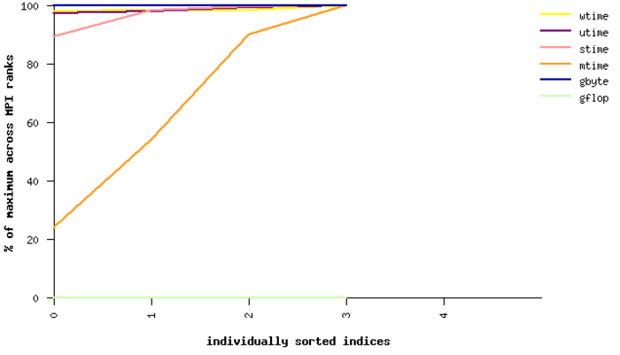
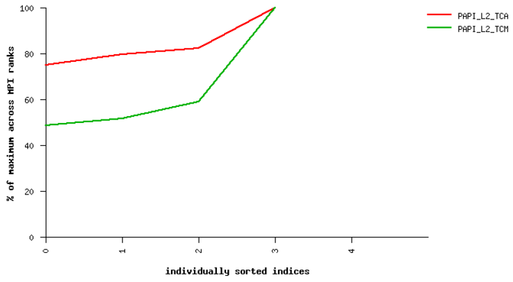
Example HTML Performance Summary
Running ipm_parse -html <xmlfile> on the generated xml file will produce an
HTML document that includes summary performance numbers and automatically
generated figures. Some examples are shown here.
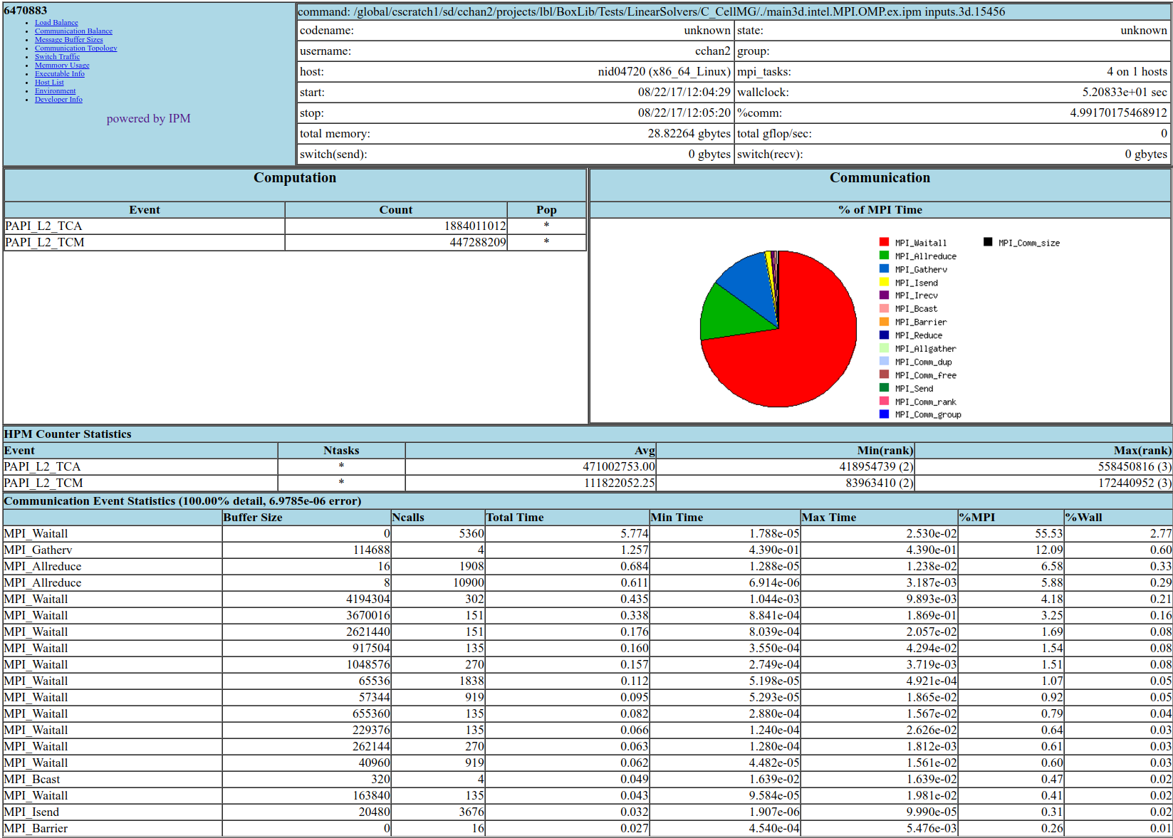
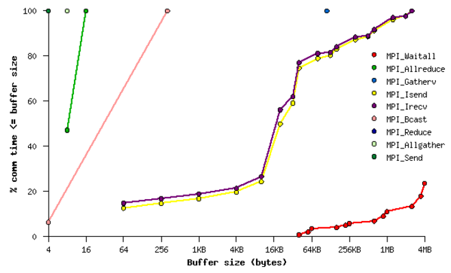
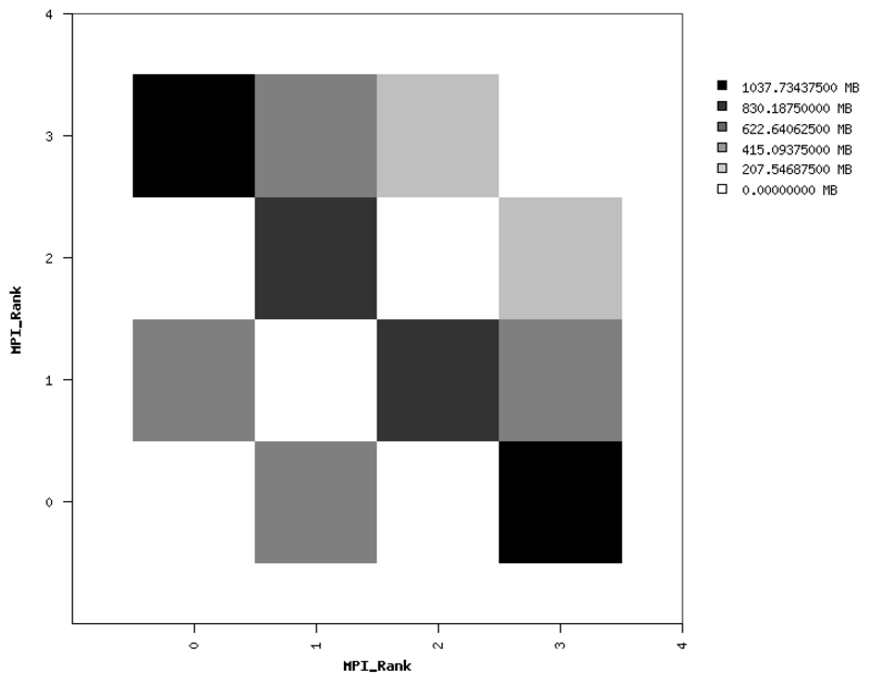
Fig. 21 Sample performance summary generated by IPM
|
|
Timings
|
PAPI Counters
|
|
|
MPI Time by Function
|
MPI Time by Message Size
|
|
(left) Point-to-Point Communication Volume
|
Nsight Systems
The Nsight Systems tool provides a high-level overview of your code, displaying the kernel launches, API calls, NVTX regions and more in a timeline for a clear, visual picture of the overall runtime patterns. It analyzes CPU codes or CUDA-based GPU codes and is available on Summit and Cori in a system module.
Nsight Systems provides a variety of profiling options. This documentation will cover the most commonly used options for AMReX users to keep track of useful flags and analysis patterns. For the complete details of using Nsight Systems, refer to the Nsight Systems official documentation.
Profile Analysis
The most common use case of Nsight Systems for AMReX users is the creation of a qdrep file that is viewed in the Nsight Systems GUI, typically on a local workstation or machine.
To generate a qdrep file, run nsys with the -o option:
nsys profile -o <file_name> ${EXE} ${INPUTS}
AMReX’s lambda-based launch system often makes these timelines difficult to parse, as the kernels
are mangled and difficult to decipher. AMReX’s Tiny Profiler includes NVTX region markers,
which can be used to mark the respective section of the Nsight Systems timeline. To include AMReX’s
built-in Tiny Profiler NVTX regions in Nsight Systems outputs, compile AMReX with TINY_PROFILE=TRUE.
Nsight Systems timelines only profile a single, contiguous block of time. There are a variety of methods to specify the specific region you would like to analyze. The most common options that AMReX users may find helpful are:
Specify an NVTX region as the starting point of the analysis.
This is done using -c nvtx -p "region_name@*" -e NSYS_NVTX_PROFILER_REGISTER_ONLY=0, where region_name
is the identification string for the NVTX region. The additional environment variable,
-e ... is needed because AMReX’s NVTX region names currently do not use a registered string.
TinyProfiler’s built-in NVTX regions use the same identification string as the timer itself. For
example, to start an analysis at the do_hydro NVTX region, run:
nsys profile -o <file_name> -c nvtx -p "do_hydro@*" -e NSYS_NVTX_PROFILER_REGISTER_ONLY=0 ${EXE} ${INPUTS}
This will profile from the first instance of the specified NVTX region until the end of the
application. In AMReX applications, this can be helpful to skip initialization and analyze the
remainder of the code. To only analyze the specified NVTX region, add the flag -x true, which
will end the analysis at the end of the region:
nsys profile -o <file_name> -c nvtx -p "do_hydro@*" -x true -e NSYS_NVTX_PROFILER_REGISTER_ONLY=0 ${EXE} ${INPUTS}
Again, it’s important to remember that Nsight Systems only analyzes a single contiguous block of time. So, this will only give you a profile for the first instance of the named region. Plan your Nsight Systems analyses accordingly.
Specify a region with CUDA profiler function calls.
This requires manually altering your source code, but can provide better specificity in what you analyze.
Directly insert cudaProfilerStart\Stop around the region of code you want to analyze:
cudaProfilerStart();

// CODE TO PROFILE

cudaProfilerStop();
Then, run with -c cudaProfilerApi:
nsys profile -o <file_name> -c cudaProfilerApi ${EXE} ${INPUTS}
As with NVTX regions, Nsight Systems will only profile from the first call to cudaProfilerStart()
to the first call to cudaProfilerStop(), so be sure to add these markers appropriately.
Nsight Systems GUI Tips
When analyzing an AMReX application in the Nsight Systems GUI using NVTX regions or
TINY_PROFILE=TRUE, AMReX users may find it useful to turn on the feature “Rename CUDA Kernels by NVTX”. This will change the CUDA kernel names to match the inner-most NVTX region in which they were launched instead of the typical mangled compiler name. This will make identifying AMReX CUDA kernels in Nsight Systems reports considerably easier.This feature can be found in the GUI’s drop-down menu, under:
Tools -> Options -> Environment -> Rename CUDA Kernels by NVTX.
Nsight Compute
The Nsight Compute tool provides a detailed, fine-grained analysis of your CUDA kernels, giving details about the kernel launch, occupancy, and limitations while suggesting possible improvements to maximize the use of the GPU. It analyzes CUDA-based GPU codes and is available on Summit and Cori in system modules.
Nsight Compute provides a variety of profiling options. This documentation will focus on the most commonly used options for AMReX users, primarily to keep track of useful flags and analysis patterns. For the complete details of using Nsight Compute, refer to the Nsight Compute official documentation.
Kernel Analysis
The standard way to run Nsight Compute on an AMReX application is to specify an output file
that will be transferred to a local workstation or machine for viewing in the Nsight Compute GUI.
Nsight Compute can be told to return a report file using the -o flag. In addition, when
running with Nsight Compute on an AMReX application, it is important to turn off the floating-point
exception trap, as it causes a runtime error. So, an entire AMReX application can be
analyzed with Nsight Compute by running:
ncu -o <file_name> ${EXE} ${INPUTS} amrex.fpe_trap_invalid=0
However, this implementation should almost never be used by AMReX applications, as the analysis of
every kernel would be extremely lengthy and unnecessary. To analyze a desired subset of CUDA
kernels, AMReX users can use the Tiny Profiler’s built-in NVTX regions to narrow the scope of
the analysis. Nsight Compute allows users to specify which NVTX regions to include and exclude
through the --nvtx, --nvtx-include and --nvtx-exclude flags. For example:
ncu --nvtx --nvtx-include "Hydro()/" --nvtx-exclude "StencilA(),StencilC()" -o kernels ${EXE} ${INPUTS} amrex.fpe_trap_invalid=0
will return a file named kernels which contains an analysis of the CUDA kernels launched inside
the Hydro() region, ignoring any kernels launched inside StencilA() and StencilC().
When using the NVTX regions built into AMReX’s TinyProfiler, be aware that the application must be built
with TINY_PROFILE=TRUE and the NVTX region names are identical to the TinyProfiler timer names.
Note that the / must be appended to the TinyProfiler timer name specified with --nvtx-include
because TinyProfiler sets NVTX push/pop regions, as described in the Nsight Compute official documentation on
NVTX Filtering.
Another helpful flag for selecting a reasonable subset of kernels for analysis is the -c option. This
flag specifies the total number of kernels to be analyzed. For example:
ncu --nvtx --nvtx-include "GravitySolve()/" -c 10 -o kernels ${EXE} ${INPUTS} amrex.fpe_trap_invalid=0
will only analyze the first ten kernels inside the GravitySolve() NVTX region.
For further details on how to choose a subset of CUDA kernels to analyze, or to run a more detailed analysis, including CUDA hardware counters, refer to the Nsight Compute official documentation.
Roofline
As of version 2020.1.0, Nsight Compute has added the capability to perform roofline analysis on CUDA kernels to describe how well a given kernel is running on a given NVIDIA architecture. For details on the roofline capabilities in Nsight Compute, refer to the NVIDIA Kernel Profiling Guide.
To run a roofline analysis on an AMReX application, run ncu with the flag
--section SpeedOfLight_RooflineChart. Again, using appropriate NVTX flags to limit the scope of the
analysis will be critical to achieve results within a reasonable time. For example:
ncu --section SpeedOfLight_RooflineChart --nvtx --nvtx-include "MLMG()" -c 10 -o roofline ${EXE} ${INPUTS} amrex.fpe_trap_invalid=0
will perform a roofline analysis of the first ten kernels inside the region MLMG(), and report
their relative performance in the file roofline, which can be read by the Nsight Compute GUI.
For further information on the roofline model, refer to the scientific literature, Wikipedia overview, NERSC documentation and tutorials.