Interphase Coupling

Deposition scheme

The following inputs must be preceded by “mfix.”

	Description	Type	Default
deposition_scheme	The algorithm that will be used to deposit particles quantities to the Eulerian grid. Available methods are: ‘centroid’ ‘trilinear’ ‘true-dpvm’ divided particle volume method ‘trilinear-dpvm-square’ dpvm with square filter	String	‘trilinear’
deposition_scale_factor	The deposition scale factor. Only applies to ‘true-dpvm’ and ‘trilinear-dpvm-square’ methods. Its value must be in the interval [0, dx/2], where dx is the cell edge size.	Real	1.0
deposition_diffusion_coeff	If a positive value is set, a diffusion equation with this diffusion coefficient is solved to smooth deposited quantities.	Real	-1.0

In the following subsections, the four possible deposition methods are briefly described and illustrated.

Centroid

In the centroid deposition scheme, particles’ quantities are deposited only to the Eulerian grid cell to which the particle’s center belongs.

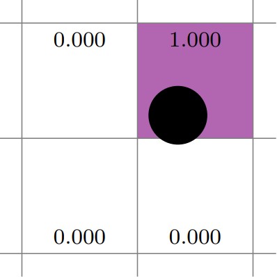
Fig. 1 Example of centroid deposition.

Trilinear

In the trilinear deposition scheme, particles’ quantities are deposited linearly to the eight Eulerian grid cells that surround its center.

Fig. 2 Example of trilinear deposition.

Divided Particle Volume Method (DPVM)

In the DPVM method, particles’ quantities are deposited to the Eulerian grid cells that they intersect, and the deposition weights are equal to the percentage of the particle’ volume that intersects the given cell.

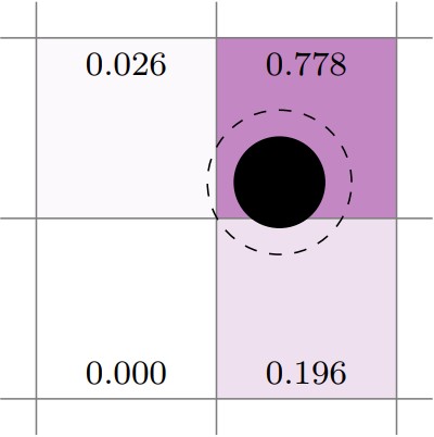
Fig. 3 Example of dpvm deposition.

Square DPVM

In the square DPVM method, particles’ quantities are deposited to the Eulerian grid similarly to the DPVM method, but with a filter applied to the deposition scheme.

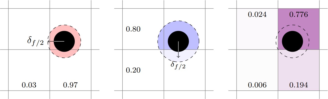
Fig. 4 Example of square dpvm deposition.

Drag

The following inputs must be preceded by “mfix.”

	Description	Type	Default
drag_type	Which drag model to use	String	None

The options currently supported in mfix are WenYu, Gidaspow, BVK2, or UserDrag.

If one of these is not specified, the code will abort with

amrex::Abort::0::"Don't know this drag type!!!

The drag models are defined in src/src_des/des_drag_K.H

If the user wishes to use their own drag model, they must

• specify mfix.drag_type = UserDrag in the inputs file

• provide the code in the ComputeDragUser routine in a local usr_drag.cpp file. An example can be found in tests/DEM06-x.

With the variables defined as follows:

/*
 *  \brief Returns: the calculated drag coefficient.
 *
 *  Inputs:
 *    EPg     - gas volume fraction
 *    Mug     - gas laminar viscosity
 *    ROpg    - gas density * EP_g
 *    vrel    - magnitude of gas-solids relative velocity
 *    DPM     - particle diameter of solids phase M
 *    DPA     - average particle diameter
 *    PHIS    - solids volume fraction of solids phases
 *    fvelx   - x component of the fluid velocity at the particle position
 *    fvely   - y component of the fluid velocity at the particle position
 *    fvelz   - z component of the fluid velocity at the particle position
 *    i, j, k - particle cell indices
 *    pid     - particle id number
 */

The WenYu model is defined as

 RE = (Mug > 0.0) ? DPM*vrel*ROPg/Mug : DEMParams::large_number;

if (RE <= 1000.0)
{
    C_d = (24.0/(RE+DEMParams::small_number)) * (1.0 + 0.15*std::pow(RE, 0.687));
}
else
{
    C_d = 0.44;
}

if (RE < DEMParams::eps) return 0.0;
return 0.75 * C_d * vrel * ROPg * std::pow(EPg, -2.65) / DPM;

The Gidaspow model is defined as

ROg = ROPg / EPg;

RE = (Mug > 0.0) ? DPM*vrel*ROPg/Mug : DEMParams::large_number;

// Dense phase - EPg <= 0.8
Ergun = 150.0*(1.0 - EPg)*Mug / (EPg*DPM*DPM) + 1.75*ROg*vrel/DPM;

// Dilute phase - EPg > 0.8
if (RE <= 1000.0)
{
    C_d = (24.0/(RE+DEMParams::small_number)) * (1.0 + 0.15*std::pow(RE, 0.687));
}
else
{
    C_d = 0.44;
}

WenYu = 0.75*C_d*vrel*ROPg*std::pow(EPg, -2.65) / DPM;

// switch function
PHI_gs = atan(150.0*1.75*(EPg - 0.8))/M_PI / DPM;

// blend the models
if (RE < DEMParams::eps) return 0.0;
return (1.0 - PHI_gs)*Ergun + PHI_gs*WenYu;

The BVK2 model is defined as

amrex::Real RE = (Mug > 0.0) ? DPA*vrel*ROPg/Mug : DEMParams::large_number;

if (RE > DEMParams::eps)
{
    oEPgfour = 1.0 / EPg / EPg / EPg / EPg;

    // eq(9) BVK J. fluid. Mech. 528, 2005
    // (this F_Stokes is /= of Koch_Hill by a factor of ep_g)
    F_Stokes = 18.0*Mug*EPg/DPM/DPM;

    F = 10.0*PHIS/EPg/EPg + EPg*EPg*(1.0 + 1.5*sqrt(PHIS));

    F += RE*(0.11*PHIS*(1.0+PHIS) - 4.56e-3*oEPgfour +
         std::pow(RE, -0.343)*(0.169*EPg + 6.44e-2*oEPgfour));

    // F += 0.413*RE/(24.0*EPg*EPg) *
    //     (1.0/EPg + 3.0*EPg*PHIS + 8.4/std::pow(RE, 0.343)) /
    //     (1.0 + std::pow(10.0, 3.0*PHIS)/std::pow(RE, 0.5 + 2.0*PHIS));

    return F*F_Stokes;
}
else
{
    return 0.0;
}

Heat Transfer Coefficient

The following inputs must be preceded by “mfix.”

	Description	Type	Default
convection_type	Which HTC model to use	String	RanzMarshall

The options currently supported in mfix are RanzMarshall (default) and Gunn. In both models the HTC is determined from a Nusslet number corelation.

The RanzMarshall Nusselt number correlation is defined as:

amrex::Real N_Nu = 2.0 + 0.6 * std::sqrt(N_Re) * std::pow(N_Pr, 0.333);

The Gunn Nusselt number correlation is defined as:

amrex::Real N_Nu =
    (7 - 10*EPg + 5*EPg*EPg)*(1 + .7*std::pow(N_Re, 0.2)*std::cbrt(N_Pr))
    + (1.33 - 2.4*EPg + 1.2*EPg*EPg)*std::pow(N_Re, 0.7)*std::cbrt(N_Pr);